June 2024 I Volume 45, Issue 2
The Robust Classical MTBF Test
June 2024
Volume 45 I Issue 2
IN THIS JOURNAL:
- Issue at a Glance
- Chairman’s Message
Conversations with Experts
- A T&E Career of Learning by Doing: A Conversation with Mr. Edward R Greer
- A Bourbon with Rusty: A Conversation with Russell L. Roberts
Values in T&E
- My T&E Career, The First 25 Years
- The Architecture Analogy in Test Planning: An example of the T&E value of 'Well-Planned'
- Values in Operational Testing
Technical Articles
- Digital Test and Evaluation: Validation of System Models as a Key Enabler
- Statistical Review of the Cyber Test Process
- The Robust Classical MTBF Test
Workforce of the Future
- Deep Learning for Autonomous Vehicles
- The K-D Tree as an Acceleration Structure in Dynamic, Three-Dimensional Ionospheric Modeling
- Optimization Engine to Enable Edge Deployment of Deep Learning Models
News
- Association News
- Chapter News
- Corporate Member News
![]()
The Robust Classical MTBF Test

Tom Roltsch
Principal Reliability Engineer
ManTech International Corporation
Herndon, VA
![]()
![]()
Abstract
For the reliability demonstration of a repairable system, testers expediently assume that the rate of occurrence of failures (ROCOF) can be modeled by a homogenous Poisson process (HPP), also called an ordinary renewal process (ORP), and therefore the times between failure, or interarrival times, are exponentially distributed with a constant mean time between failures (MTBF). This often-used test is colloquially called the “classical MTBF test” because it has been widely used by both government and industry for the past 50 years. The test is simple; operate a system for a period and the sample estimate for MTBF is the operating time divided by the number of failures. A confidence interval is applied to the sample estimate to determine the test result. This paper considers the validity of the test result if the repairable system has an increasing or decreasing MTBF, that is, a nonhomogeneous Poisson process (NHPP). Specifically, the change in consumer’s risk is analyzed if the repairable system has a decreasing MTBF (increasing ROCOF). A simple risk mitigation strategy consisting of a burn-in period equal to the threshold MTBF is also considered and found to be effective. The classical MTBF test is shown to be a robust test and a burn-in period prior to testing makes the classical MTBF test even more robust.
Keywords: Reliability test, MTBF test, RAM test, Reliability, MTBF, HPP, Power-law process, NHPP
Introduction
Reliability analysis for repairable systems is different from reliability analysis for non-repairable components. Non-repairable components fail only once. To get a sample, many components of the same type must be tested, each yielding a single data point for its time-to-failure. A best fit for the sample of times-to-failure might be an exponential distribution with constant mean time to failure (MTTF). However, testers cannot assume that the best fit distribution for a non-repairable component will be exponential; it could be Weibull, lognormal, or some other distribution.
Repairable systems fail many times and are renewed after each failure; thus, a renewal process is used to describe the reliability of a repairable system. Renewal processes have been studied from a statistics perspective since the late 1930’s with the seminal work being done by Alfred Lotka, a statistician for Metropolitan Life Insurance Company (“Lotka, Alfred J. | Encyclopedia.com,” n.d.). Lotka described the renewal process in terms of demographics (Lotka 1939). Renewal theory was further developed by other statisticians including David Blackwell who proved that, given enough time, any renewal process will become a homogenous Poisson process (HPP) (Blackwell 1948). The renewal process was used to describe the reliability of repairable systems by Harold Ascher and Harry Feingold in their 1984 book, Repairable Systems Reliability: Modelling, Inference, Misconceptions and their Causes (Ascher and Feingold 1984). The use of the renewal process to describe the reliability of repairable systems was further developed by
Maasaki Kijima leading to the generalized renewal process which includes ranking the effectiveness of a repair from minimal to perfect (Kijima 1989). Unfortunately, the generalized renewal process solutions can only be determined using Monte Carlo methods. For most repairable systems the reliability can be modeled as a homogenous Poisson process (HPP), also called an ordinary renewal process (ORP), or as a non-homogenous Poisson process (NHPP) (NIST 2012, 8.1.7.1). In an HPP the times between failure follow an exponential distribution with constant MTBF. In a NHPP the times between failure are either increasing or decreasing over time. The HPP assumes that repairs make the system “as good as new,” also called “perfect repair.” The NHPP assumes that repairs make the system “as good as old,” also called “minimal repair.” These two cases can be thought of as extremal (Modarres, Kaminskiy, and Vasiliy Krivtsov 2016, 252). Kajima’s models added a repair effectiveness factor that makes it possible to calculate reliability for repairable systems that would fail between these extremal values such as “better than old but worse than new” (Wang and Yang 2012, 1128).
Background
Using the HPP for testing the MTBF of new repairable systems, without any repair analysis, was incorporated into Department of Defense (DoD) handbooks such as Military Handbook 781 (MIL-HDBK-781), Reliability Test Methods, Plans, and Environments for Engineering Development, Qualification, and Production. While this handbook is still active and valid as guidance it cannot be referenced as a requirement in a contract. The current Reliability Standard that is authorized by DoD for use in contracts is the Government Electronics & Information Technology Association (GEIA) Standard 0009A, Reliability Program Standard for Systems Design, Development, and Manufacturing (GEIA 2019, 1). Accompanying this standard is a reliability program handbook, GEIA TAHB0009A. For reliability testing of new repairable systems the GEIA reliability program handbook refers the reader to MIL-HDBK-781 but includes a disclaimer (GEIA 2019, 335). The disclaimer is taken, almost word-for-word from the DoD Guide for Achieving Reliability, Availability, and Maintainability (DoD 2005, 4-69).
MIL-HDBK-781 test plans are based on the assumption that a constant failure rate is applicable for the equipment being tested. The constant failure rate assumption means that MTBF will be the reliability metric used for the MIL-HDBK-781 test plan. The Handbook offers numerous test plans that enable the selection of a plan that best fits the needs of the program by balancing the statistical risks (producer’s risk versus consumer’s risk) involved and the minimum level of acceptable reliability…Reliability demonstration testing to MIL-HDBK-781 is subject to limitations, which cause it to be a controversial Method. The exponential distribution assumption of a constant failure rate is one fundamental limitation.
The DoD guide gives a list of reasons, such as degradation due to various causes, why an operational system might, over its lifetime, suffer a decreasing failure rate. With enough failure data and repair data the rate of degradation could be determined. Such an analysis is lengthy and expensive but may be worthwhile in some cases where a high level of precision is needed.
A relatively quicker and easier, albeit less precise, method to verify the minimum MTBF of a new repairable system is to assume, for testing purposes only, that failure times can be modeled as an HPP and MTBF is therefore constant. The causes listed in the DoD guide for why an operational system might, over its lifetime, suffer a decreasing failure rate are all valid, however, none of these long term, real world operational effects challenge the test assumption of a constant failure rate. The test is only designed to verify that the system, as delivered, meets at least the threshold MTBF requirement at a predetermined confidence level. The HPP model serves well for that purpose. After a system is fielded there may be environmental and usage factors that cause early wear out of some components and imperfect repair techniques that cause further failures. So, an estimate for the lifetime MTBF of a system using the HPP model may be high, and some degradation must be expected. In this paper it is shown that degrading systems, that is, systems with MTBF that is decreasing over time, pose only a small test risk when using the HPP model to design a test.
In this author’s opinion the disclaimer statement in both the GEIA handbook and DoD guide is flawed because the tests described in MIL-HDBK-781 are perfectly adequate for qualification/acceptance testing of most new repairable systems. Moreover, the test techniques described in MIL-HDBK-781 are widely used in acquisition practice to this day, both for individual systems and for fleets of systems. That means that each year billions of dollars’ worth of equipment is evaluated using these tests. Therefore, it is important for the test community to know that these tests are robust. In this paper the fixed duration test, also called the “classical MTBF test,” is discussed.
Technically, a software application does not follow a renewal process, at least not an ordinary renewal process because software cannot be repaired, it requires a configuration change. Thus, each time a software application is tested after a “fix” it is a new configuration that, hopefully, is more reliable than the previous configuration. This process is more akin to reliability growth, which could be modeled as an NHPP with MTBF that is increasing over time. However, a software application can be treated as one component of an enterprise information technology (IT) system. If an IT system has numerous software application components and numerous hardware components, then the resulting system-of-systems may follow an ordinary renewal process.
The Classical MTBF Test
For the reliability demonstration of a repairable system, testers expediently assume that the system can be modeled as an HPP so the rate of occurrence of failures (ROCOF) is constant and therefore the times between failure, or interarrival times, are exponentially distributed with a constant MTBF. The assumption of constant MTBF, for the purpose of testing a new repairable system, is a good assumption. It allows a robust fixed-length test to be designed, with low consumer and producer risks.
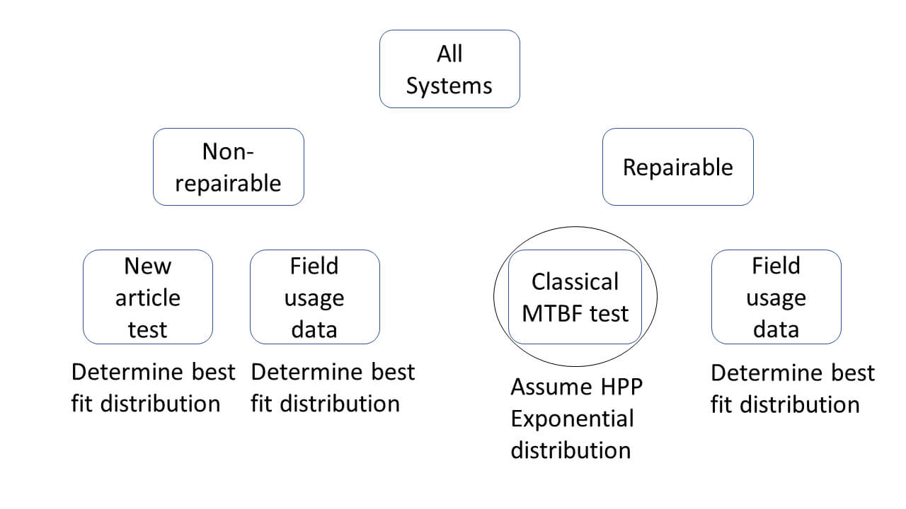 Figure 1. Correct use of classical MTBF Test is for new, repairable systems only
This often-used inferential statistics test is colloquially called the classical MTBF test because it has been in use by both government and industry for the past 50 years. The test is simple: operate a system for a period and the sample estimate for MTBF is the operating time divided by the number of failures. An exact confidence interval is applied to the sample estimate using the chi-squared distribution as a pivot to determine the test result. The classical MTBF test with a one-sided lower confidence interval as the test result is described in MIL-HDBK-338, MIL-HDBK-781 and MIL-HDBK-189 (“Confidence Bounds on the Mean Time between Failure (MTBF) for a Time-Truncated Test” n.d.). The confidence interval is calculated using the chi-squared distribution, with two times the number of failures plus two failures for the degrees of freedom. Adding two failures to the degrees of freedom in the calculation of the chi-squared probability allows a solution when there are zero failures and makes the test more conservative. For U.S. Government testing, often an 80% confidence level is used as a trade-off between cost and risk. The classical MTBF test is based on probability, it is not a measurement of MTBF or reliability, thus it has only two outcomes: the MTBF is verified to be at least the threshold value at the specified confidence level, or it is not. In general, systems that are the same make and model will have similar attributes including similar MTBF and reliability attributes. Therefore, this test can be used for a single system or a fleet of systems.
Even if the interarrival times for the system are not exponentially distributed, the test results are correct in most cases. Moreover, a period of burn-in prior to the test will make the test even more robust as it will decrease the probability that a system with MTBF that is decreasing over time will pass the classical MTBF test. Figure 1 illustrates the correct use of the classical MTBF test for a new repairable system. It is a good assumption that MTBF is constant for testing a new repairable system. In most other cases it would not be assumed that the MTTF or MTBF is constant.
The acronym MTBF is typically used only for repairable systems with constant ROCOF (constant MTBF). Since this is a paper about MTBF testing, the ROCOF will not be used and instead instantaneous values of MTBF will be used. In all figures instantaneous MTBF values are used which are 1/ROCOF at time t. If the MTBF is increasing or decreasing then every time, t, will have a different value for MTBF. The lifetime MTBF, also called useful life MTBF or design life MTBF, is an average of all the instantaneous MTBF values over the system lifetime. Of course, if the MTBF is constant then the instantaneous MTBF is the same at every time, t, and is equal to the lifetime MTBF.
The classical MTBF test is often used in government acquisition programs to verify that a new repairable system’s lifetime MTBF will be at least as great as the threshold requirement. It is a predictive test and is based on probabilities that are calculated from the HPP model, that is, the assumption that the MTBF will be constant over the system’s useful life. But what happens if the MTBF is not constant over the system’s useful life? An MTBF that is increasing over time is not a risk to the consumer, however, if the MTBF is decreasing over time, then the MTBF could be great enough during the test period to allow the system to pass the test while the MTBF over the system lifetime could be lower than the threshold requirement. This fact is sometimes asserted as a weakness for the classical MTBF test.
As will be shown below, the classical MTBF test is robust in that only a small subset of decreasing MTBF systems will have MTBF that is great enough during the test period to allow the system to pass the test while the MTBF over the system lifetime could be lower than the threshold requirement. Moreover, an operating period, or burn-in period, prior to performing the classical MTBF test further reduces the probability that any decreasing MTBF system with lifetime MTBF below the threshold requirement will pass the test and makes the classical MTBF test even more robust.
A classical MTBF test can be designed to allow a maximum number of failures for a predetermined time interval, which is called a time-truncated test. Unlike a failure-truncated test or a sequential test, the time-truncated test has a definite test time. This distinction makes the time-truncated test advantageous because a known amount of expensive test time can be scheduled in advance. Thus, in practice, the time-truncated classical MTBF test is the preferred method for many programs. If the system operates for the predetermined test time with fewer than the maximum number of allowed failures, then the MTBF is verified to meet at least the threshold requirement at a predetermined confidence level.
The system could have no failures at all during the test and the MTBF is still verified to be at least as great as the threshold requirement without witnessing a system failure. In fact, combined with a maintenance demonstration to verify mean time to repair (MTTR) and good estimates for logistics delay time and the frequency and duration of preventive maintenance, a good estimate for minimum operational availability can be made without witnessing a single system failure–thus exemplifying the efficiency of statistical test techniques.
The consumer’s risk for a time-truncated classical MTBF test at the 80% confidence level is calculated such that the probability of passing the test for a system with lifetime MTBF equal to the threshold requirement will be 20%. Often, the producer’s risk is desired to be about the same as the consumer’s risk, thus the calculation of the test time also accounts for 80% power level. For the classical MTBF test both producer and consumer risk can be set in advance and are dependent on the discrimination ratio, d. Let mt be the threshold MTBF requirement and mo be the objective MTBF requirement, then the discrimination ratio, d, is defined as in Equation (1).
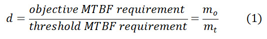
Although the discrimination ratio can vary, typical values are between 2 and 3. Table 1 shows the test length, τ, needed to achieve approximately 20% consumer and producer risks for discrimination ratios ranging from 1.5 to 3.5. The test length, τ, is expressed in multiples of the threshold MTBF requirement, mt.
Table 1. Test length for the classical MTBF test in multiples of mt
|
Discrimination ratio, d = mo/mt |
Test length, τ, to achieve consumer and producer risk approximately 20% | Number of failures allowed to verify MTBF threshold requirement |
| 1.5 | 19.2(mt) | 15 |
| 2 | 7.906(mt) | 5 |
| 2.5 | 5.515(mt) | 3 |
| 3 | 4.279(mt) | 2 |
| 3.5 | 2.994(mt) | 1 |
The Nonhomogeneous Poisson Process (NHPP) Power-law Model
The power-law model, which is an NHPP with an underlying Weibull distribution, can be used to describe most systems that have an increasing or decreasing ROCOF (NIST 2012, 8.1.7.2). Exceptions exist, and it is theoretically possible for the underlying distribution to be any distribution (Krivtsov 2007, 560). For example, a system that initially has an MTBF that increases with time but later decreases with time could not be modeled by a power-law, but such a system would be out of the norm. For generality, the power-law model will be used in this paper. The power-law model has instantaneous MTBF equal to the inverse of the ROCOF. The ROCOF is symbolized as ρ(t), with scale parameter, a, and shape parameter, b, thus instantaneous MTBF is the inverse, or 1/ρ(t), as shown in Equation (2) (NIST 2012, 8.1.7.2).
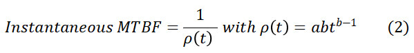
Both the scale parameter and shape parameter are constants, but the values of both ρ(t) and instantaneous MTBF change over time. If the shape parameter, b, is less than 1 the MTBF increases over time. If the shape parameter, b, is greater than 1 then the MTBF decreases over time. If the shape parameter, b, is equal to 1 then the MTBF is constant. Graphically, the MTBF over time is curved for the power-law model while the MTBF over time for the HPP model is a flat, horizontal line representing the constant MTBF. Figure 2 shows the instantaneous MTBF for single system with the following: mt = 100, mo = 200, a = 1/mo, d = 2, test length is 7.906mt. The curves show parameter b = 0.99 and b = 1.1; the flat, horizontal lines for b = 1 represent constant MTBF. Note that the units of MTBF could be hours, miles, rounds fired, etc. For this paper the units are considered to be hours.
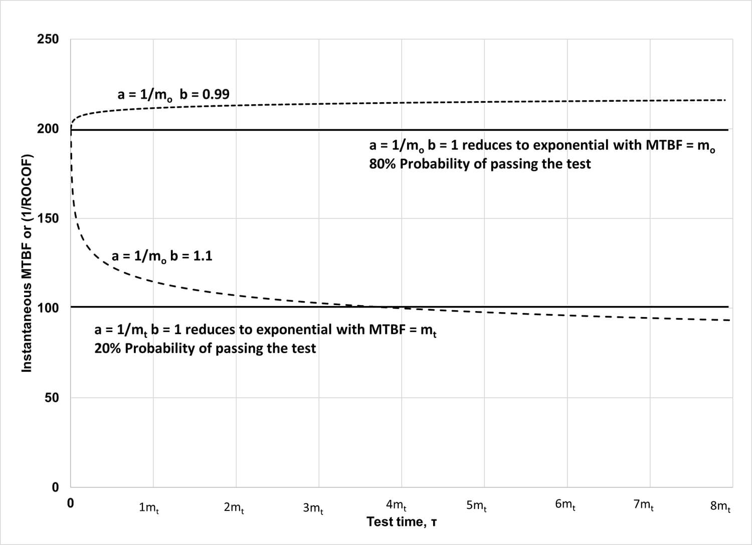
Figure 2. Graphs of the power law with three values of b for a = 1/mo and one value for a = 1/mt
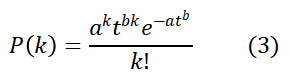
The probability of having exactly k failures in a time interval, t, for the power-law model is given by Equation (3) (Ebeling 2010, 233).
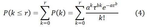
If the time, t, is the test length, τ, and the number of failures allowed to pass the test is r, then the probability of passing the test is shown in Equation (4).
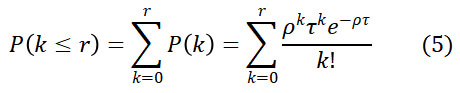
When b = 1, the ROCOF is equal to a and is constant. Equation (4) reduces to the probability of passing the test for the HPP model as in Equation (5).
We would like to know the probability of passing a test that is designed under the assumption of the HPP model when the system has decreasing MTBF, that is, power-law model. This will indicate the robustness of the classical MTBF test. Robustness being the sensitivity of the test result to the actual distribution being different from the assumed distribution. Therefore, to check the robustness of the classical MTBF test we need to see if the consumer’s risk is increased when the assumed distribution, with b = 1, differs from the actual distribution, with b > 1. We don’t need to check for the case where b < 1 because that would be an increasing MTBF which does not increase the consumer’s risk.
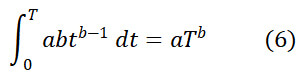
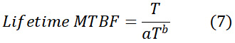
Since the MTBF is changing over time, the system’s useful life, T, must be specified to calculate a lifetime MTBF for the power-law model. The lifetime MTBF for the power-law model is calculated by dividing the system’s useful life, T, by the expected number of failures. The expected number of failures is the integral of the ROCOF from time 0 to the end of the system’s useful lifeas shown in Equation (7). The integral of the ROCOF is shown in Equation (6) for completeness.
The lifetime MTBF for the power-law model is shown in Equation (7).
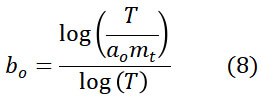
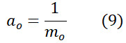
In mathematical terms, let’s examine what happens to consumer risk if b > 1 and a test is designed based on the assumption that b = 1 when the discrimination ratio is equal to 2. For a given value of a, which we will call ao, there is a value of b, which we will call bo, that corresponds to a lifetime MTBF equal to the threshold requirement. Using the values for ao and bo in the equation for the NHPP power-law probability of passing the test gives the probability that a system with lifetime MTBF equal to mt will pass the test. The value of bo can be calculated as shown in Equation (8). The math works nicely if we set the value of ao based on the objective MTBF requirement, for example, ao = 1/mo as shown in Equation (9).
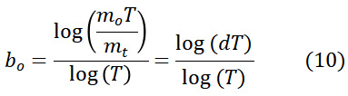
With ao set to the reciprocal of the objective MTBF requirement substitute 1/mo for ao in Equation (8) to get Equation (10) which shows that when ao = 1/mo then bo is determined only by the discrimination ratio and the system lifetime:
All b values greater than bo will have lifetime MTBF less than the threshold requirement and lesser probability of passing the test. All b values less than bo will have lifetime MTBF greater than the threshold requirement which will not increase consumer’s risk. For a values less than ao, the system would need to have a steeply declining MTBF to have a lifetime MTBF less than the threshold requirement. Such a system would likely be identified during developmental or early operational testing. Thus, an ao value equal to the reciprocal of the objective MTBF requirement and the associated bo value give a reasonable maximum for consumer’s risk. The maximum is calculated as the consumer’s risk for a system that has exactly mt for lifetime MTBF. A lifetime MTBF of exactly mt does not increase consumer’s risk, but a lifetime MTBF less than mt does increase consumer risk. For a single system the maximum consumer’s risk is given by Equation (11).
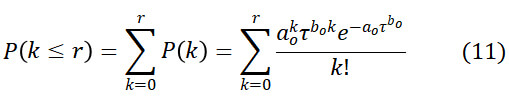 Figure 3 shows that, for a given a value, such as ao = 1/mo, only a subset of b values exist such that the probability of passing the test can be greater than 20% while the system has a lifetime MTBF less than the threshold requirement. The range of b values that can increase consumer’s risk are shown in red. It is evident from Figure 3 that when ao = 1/mo and the discrimination ratio is 2 for a single system under test with lifetime of 60,000 hours and MTBF objective requirement equal to 200 hours, the range of b values that increase consumer’s risk is from 1.063 to 1.104. All b values less than bo = 1.063 will have lifetime MTBF greater than the threshold requirement and all b values greater than 1.104 will have less than 20% chance of passing the test. This subset of b values in red from 1.063 to 1.104 are the only b values that increase the consumer’s risk when using the classical MTBF test to verify the MTBF of a new repairable system. Thus, the classical MTBF is a robust test. That is, in most cases the consumer’s risk and the result of the test is indifferent to whether the MTBF is increasing, decreasing or constant.
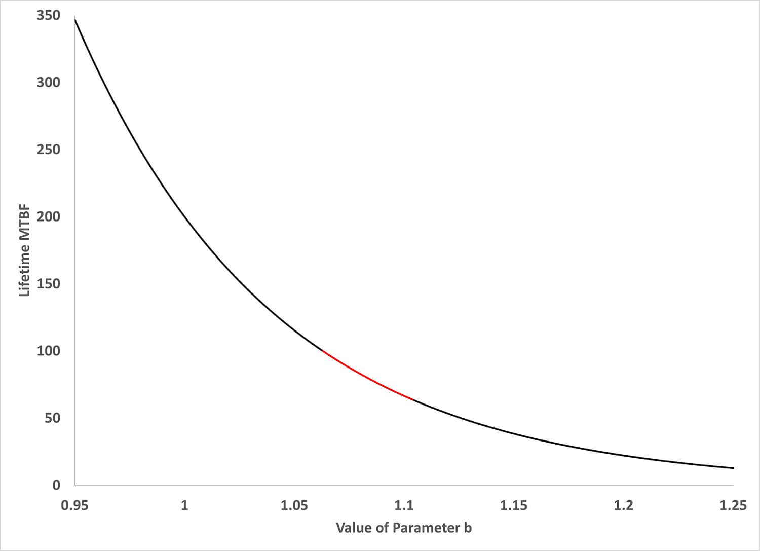 Figure 3. For ao = 1/mo with d = 2, lifetime 60,000 hours, MTBF objective requirement 200 hours, the range of b values that increase consumer’s risk is shown in red
While it is difficult to identify a “typical system,” the system represented in Figure 3 represents a nearly worst-case system. The threshold MTBF is low, and the lifetime is high. A more typical system might have an MTBF threshold requirement of 500 hours and objective requirement of 1000 hours. A realistic lifetime might be represented by 16 hours of daily operation every day for 5 years or about 29,200 hours. Figure 4 shows such a system. The small range of 0.017, or from 1.067 to 1.084, are the only values of b that increase consumer’s risk beyond 20%.
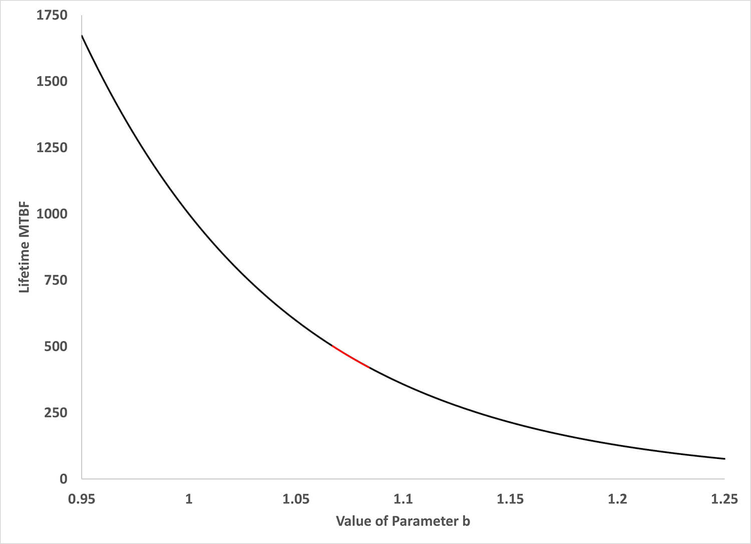 Figure 4. For ao = 1/mo with d = 2, lifetime 29,200 hours, MTBF objective requirement 1000 hours, the range of b values that increase consumer’s risk is shown in red
Further Reduction of Consumer’s Risk from Burn-in
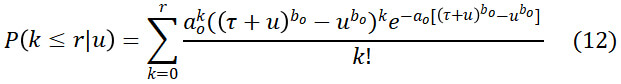
For the subset of b values that increase consumer’s risk when the repairable system has decreasing MTBF, the probability of passing the test, and therefore the consumer’s risk, is reduced by a burn-in period of length u. If the system has constant MTBF then the burn-in period has no effect on the probability of the system passing the classical MTBF test. The burn-in period can be any activity that operates the system such as an operational assessment prior to performing the classical MTBF test. Equation (12) shows the probability of passing the test after a burn-in period of length u (Ebeling 2010, 230).
 Notice that the decreasing exponential in equation 12, dominates the equation. If τ, the test time, or u, the burn-in time is increased then the probability of a decreasing MTBF system passing the test will decrease no matter what the other parameters may be. Therefore, the longer the burn-in period, the more the consumer’s risk posed by a decreasing MTBF system is reduced. However, it would be impractical to burn-in the system long enough to eliminate the consumer’s risk posed by a decreasing MTBF system. Figures 5 and 6 show for a worst-case system and a typical system, respectively, how a burn-in period equal to mt decreases the range of b values that can increase consumer risk. The black vertical line on both graphs shows the change in the range due to burn-in. The effect of burn-in is not just lowering the consumer risk, the lowest possible MTBF values, on the left side of the range, are eliminated. For this reason, a burn-in period prior to performing a classical MTBF test should be considered a best practice.
Figure 5 shows the decrease in range of b values that increase consumer’s risk due to a burn-in period, u, equal to the threshold MTBF requirement, mt, for a single system with ao = 1/mo and d = 2 with lifetime of 60,000 hours and objective MTBF requirement 200 hours. The black vertical line shows the upper range limit for b after burn-in. The range of b values that increases consumer’s risk is reduced from 1.063 to 1.104 to 1.063 to 1.099. The system in Figure 5 is near a worst-case.
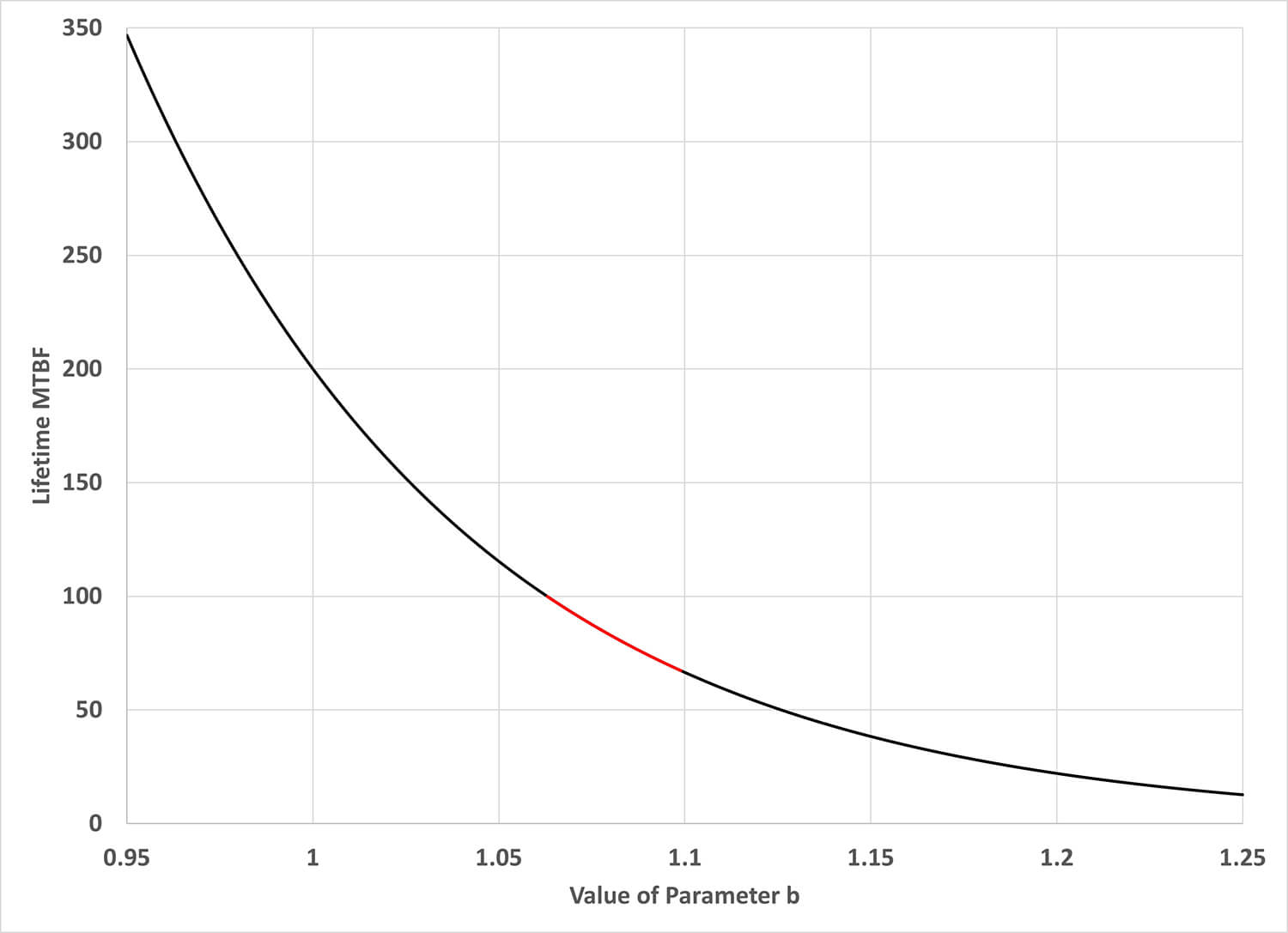 Figure 5. For ao = 1/mo with d = 2, lifetime 60,000 hours, MTBF objective requirement 200 hours, the range of b values that increase consumer’s risk after burn-in is shown in red
Figure 6 shows the decrease in range of b values that increase consumer’s risk due to a burn-in period, u, equal to the threshold MTBF requirement, for a single system with ao = 1/mo and d = 2. The black vertical line shows the upper range limit for b after burn-in. The system in Figure 6 is a typical case with MTBF threshold requirement of 500 hours and objective requirement of 1000 hours and lifetime of 29,200 hours. The range of b values that increases consumer’s risk is reduced from 1.067 to 1.084 to 1.067 to 1.080.
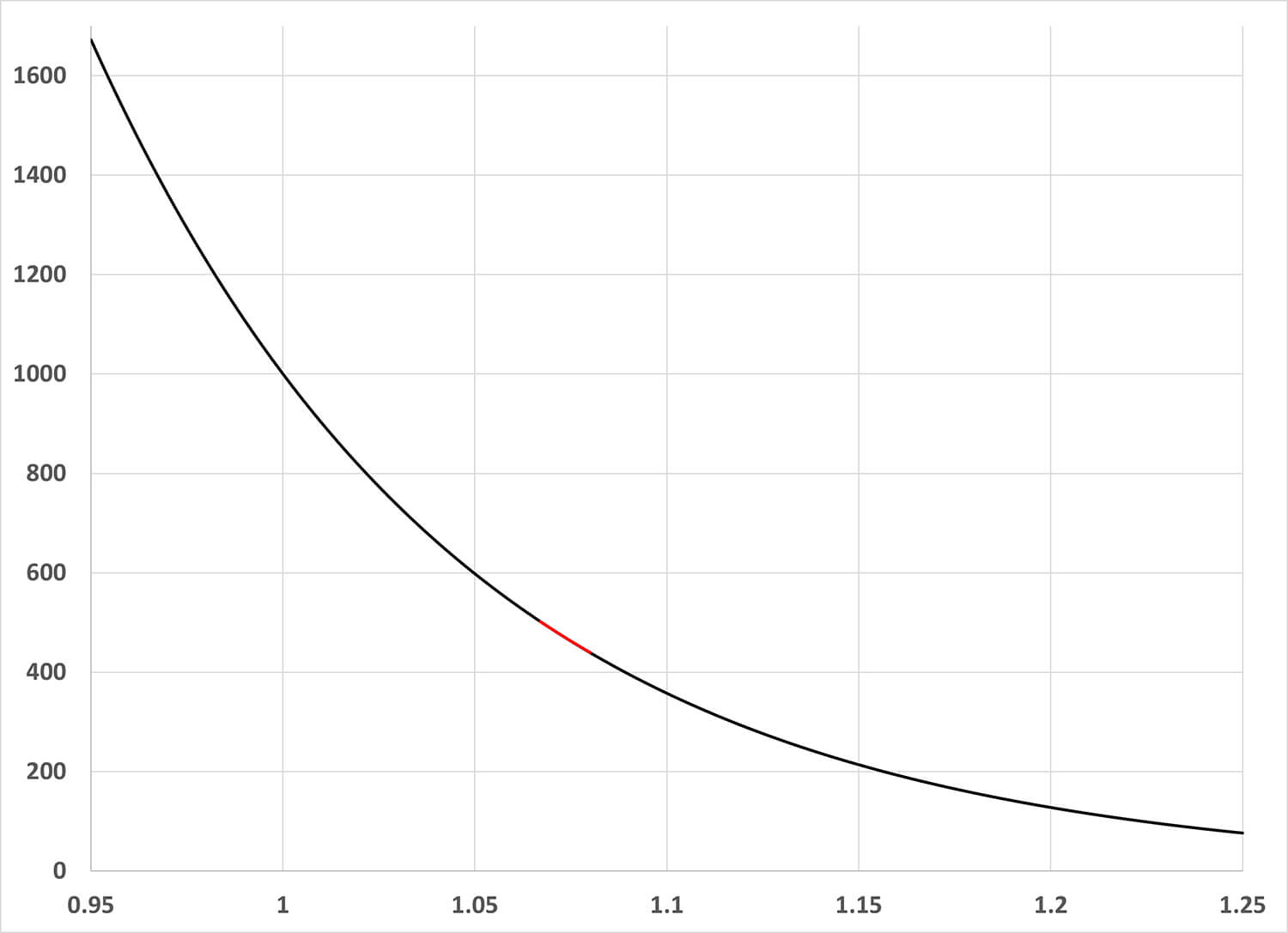 Figure 6. For ao = 1/mo with d = 2, lifetime 29,200 hours, MTBF objective requirement 1000 hours, the range of b values that increase consumer’s risk after burn-in is shown in red
If a system has decreasing MTBF according to the power-law model then for any given value of the parameter, a, there will be a small subset of b values that increases the consumer’s risk. Table 2 shows the b values that increase consumer’s risk for the given a value in the test of a single system with discrimination ratio equal to 2, mo = 200, ao = 1/mo and a useful life of 600mt. The example system in Table 2 shows the values for a nearly worst-case system due to the long useful lifetime and low threshold MTBF requirement, most other systems would have a smaller range of b values that increase consumer’s risk.
For a given parameter, a, the parameter, b, could theoretically take any value. Realistically, it would be unusual for any system to have its b parameter outside the range 0.950 to 1.250. Outside this range the MTBF would be increasing or decreasing very rapidly over time. From 0.950 to 1.250 is a range of 300 possible, realistic b values, expressed to three decimal places, for any given a value. The rightmost column in Table 2 shows the proportion of systems in this range with b values that increase consumer’s risk after burn-in. For example, at ao = 1/mo there are 36 b values that increase consumer’s risk after burn-in within the range of 300 realistically possible b values, or 12%. Therefore, 88% of repairable systems with discrimination ratio equal to 2, a useful life of 600mt, mo = 200 and ao = 1/mo or greater, would not cause any increase in consumer’s risk when using the classical MTBF test with a burn-in period equal to the threshold MTBF requirement regardless of the value of the parameter, b.
Table 2. Parameter b values that increase consumer’s risk for nearly worst-case system
|
ao |
b values that increase consumer’s risk, bo is the low value |
b values that increase consumer’s risk after burn-in of u = mt |
Maximum consumer’s risk at bo |
Maximum consumer’s risk at bo after burn-in of u = mt |
Proportion of b values between b = 0.950 and b = 1.250 |
| 1/1.25mt | 1.019 to 1.034 | 1.019 to 1.032 | 28% | 27% | 4.3% |
| 1/1.5mt | 1.037 to 1.061 | 1.037 to 1.058 | 33% | 32% | 5.6% |
| 1/mo | 1.063 to 1.104 | 1.063 to 1.099 | 44% | 42% | 12% |
The author considers it unlikely that any repairable system with ao parameter equal to 1/3mt or less, that could also have a lifetime MTBF less than mt could emerge from the design and development process. Such a system would have an exorbitant rate of decrease in MTBF over time.
Table 3 shows the same information as Table 2 but for a typical system with MTBF threshold requirement of 500 hours and objective requirement of 1000 hours and lifetime 29,200 hours.
Table 3. Parameter b values that increase consumer’s risk for a typical system
|
ao |
b values that increase consumer’s risk, bo is the low value |
b values that increase consumer’s risk after burn-in of u = mt |
Maximum consumer’s risk at bo |
Maximum consumer’s risk at bo after burn-in of u = mt |
Proportion of b values between b = 0.950 and b = 1.250 |
| 1/1.25mt | 1.022 to 1.027 | 1.022 to 1.026 | 23% | 22% | 1.3% |
| 1/1.5mt | 1.039 to 1.049 | 1.039 to 1.047 | 26% | 25% | 2.6% |
| 1/mo | 1.067 to 1.084 | 1.067 to 1.080 | 31% | 29% | 4.3% |
Table 3 shows that for a lifetime of 29,200 hours, d = 2, mo = 1000 and ao = 1/mo there are only thirteen b values that increase consumer’s risk after burn-in within the range of 300 realistically possible b values, or about 4%. Therefore, about 96% of such typical repairable systems with ao = 1/mo or greater would not cause any increase in consumer’s risk when using the classical MTBF test with a burn-in period equal to the threshold MTBF requirement regardless of the value of the parameter b. Of course, if the value of b is 1, as assumed, then there is no increase in consumer’s risk. If the value of b is less than 1, then there is no increase in consumer’s risk. If the value of b is greater than 1, then for about 96% of typical systems there is no increase in consumer’s risk. That is a robust test!
Conclusion
For MTBF testing of new repairable systems both the reliability requirement and the reliability acceptance test can use mean time between failures (MTBF) based on the assumption that a new repairable system will have times between failures that are exponentially distributed over the useful life of the system. The classical MTBF test is a robust test because, for a given value of the NHPP power-law parameter, a, only a small subset of values for the parameter b will increase the consumer’s risk. The MTBF tests described in MIL-HDBK-781A all use the assumption that interarrival times between failures can be described by the exponential distribution (constant MTBF). Here it has been shown that, at least for the fixed duration test of a single system, the classical MTBF test is robust for systems that have increasing, decreasing, or constant failure rate.
In this paper a single system with discrimination ratio equal to 2 under a classical MTBF test with 20% consumer and producer risks (80% confidence and 80% power) was considered. When testing multiple systems of the same make and model simultaneously and aggregating the operating time and number of failures, the test times will be shorter which will increase the consumer’s risk posed by a decreasing MTBF system. When testing systems with high threshold MTBF or at confidence levels greater than 80% the test times will be longer which will decrease the consumer’s risk posed by a decreasing MTBF system. For most systems the classical MTBF test will give robust results. Any burn-in period prior to performing the classical MTBF test will make the classical MTBF test even more robust.
Those industry practitioners and academic researchers who have reliability work where the classical MTBF test is insufficient, please email the author and consider publishing test articles documenting the exceptions and how to deal with these.
For all systems, a test period that is long enough to include approximately 30 failures and the corresponding analysis of the repairs will produce the best approximation of the ROCOF. However, when a relatively short test is needed to qualify a new, repairable system the classical MTBF test will give a robust result for most systems.
References
Ascher, Harold E. 1968. “Evaluation of Repairable System Reliability Using the ‘Bad-As-Old’ Concept.” IEEE Transactions on Reliability R-17 (2): 103–10. https://doi.org/10.1109/tr.1968.5217523.
Ascher, Harold, and Harry Feingold. 1984. Repairable Systems Reliability.
Barlow, Richard E, and Frank Proschan. 1967. “Exponential Life Test Procedures When the Distribution Has Monotone Failure Rate.” Journal of the American Statistical Association 62 (318): 548–60. https://doi.org/10.1080/01621459.1967.10482928.
Blackwell, David. 1948. “A Renewal Theorem.” Duke Mathematical Journal 15 (1). https://doi.org/10.1215/s0012-7094-48-01517-8.
Ebeling, Charles E. 2010. An Introduction to Reliability and Maintainability Engineering. Long Grove: Waveland.
Government Electronics & Information Technology Association (GEIA). 2019. Reliability Program Handbook TAHB0009A. GEIA.
Institute of Electrical and Electronics Engineers (IEEE). 2016. IEEE 1633, Recommended Practice on Software Reliability. IEEE. doi: 10.1109/IEEESTD.2017.7827907
Lotka, A.J. 1939. “A Contribution to the Theory of Self-renewing Aggregates, with Special Reference to Industrial Replacement.” Annals of Mathematical Statistics 10, 1–25. doi: 10.1214/aoms/1177732243
“Lotka, Alfred J. | Encyclopedia.com.” n.d. Www.encyclopedia.com. https://www.encyclopedia.com/social-sciences/applied-and-social-sciences-magazines/lotka-alfred-j.
Krivtsov, Vasily. 2007. “Practical Extensions to NHPP Application in Repairable System Reliability Analysis.” Reliability Engineering & System Safety. Volume 92, Issue 5. https://doi.org/10.1016/j.ress.2006.05.002
Kijima, Masaaki. 1989. “Some Results for Repairable Systems with General Repair.” Journal of Applied Probability 26 (1): 89–102. https://doi.org/10.2307/3214319
Modarres, Mohammad, Mark P Kaminskiy, and Vasiliy Krivtsov. 2016. Reliability Engineering and Risk Analysis. CRC Press.
Montagne, Ernest R., and Nozer D. Singpurwalla. “Robustness of Sequential Exponential Life-Testing Procedures.” Journal of the American Statistical Association 80, no. 391 (1985): 715–19. https://doi.org/10.2307/2288490.
NIST/SEMATECH e-Handbook of Statistical Methods, http://www.itl.nist.gov/div898/handbook/, April 2012.
“Confidence Bounds on the Mean Time between Failure (MTBF) for a Time-Truncated Test.” n.d. Quanterion Solutions Incorporated. Accessed May 17, 2024. https://www.quanterion.com/confidence-bounds-on-the-mean-time-between-failure-mtbf-for-a-time-truncated-test/#:~:text=In%20this%20approach%2C%20MIL-HDBK-338%2C%20MIL-HDBK-781%20and%20MIL-HDBK-189%20all.
Roltsch, Tom. “The Robust Classical MTBF Test.” Conference presentation at 2023 7th International Conference on Reliability Engineering, Bologna, Italy, November 23, 2023.
Ross, Sheldon M. 2014. “Renewal Theory and Its Applications.” Elsevier EBooks, January, 409–79. https://doi.org/10.1016/b978-0-12-407948-9.00007-4.
Smith, Walter L. 1958. “Renewal Theory and Its Ramifications.” Journal of the Royal Statistical Society. Series B (Methodological) 20 (2): 243–302. http://www.jstor.org/stable/2983891.
U.S. Department of Defense Guide for Achieving Reliability, Availability, and Maintainability, 2005.
U.S. Department of Defense, MIL-HDBK-781A, Reliability Test Methods, Plans, and Environments for Engineering Development, Qualification, and Production, 1996.
Wang, Zhi-Ming, and Jian-Guo Yang. 2012. “Numerical Method for Weibull Generalized Renewal Process and Its Applications in Reliability Analysis of NC Machine Tools.” Computers & Industrial Engineering 63 (4): 1128–34. https://doi.org/10.1016/j.cie.2012.06.019.
Zelen, M., and Mary C. Dannemiller. “The Robustness of Life Testing Procedures Derived from the Exponential Distribution.” Technometrics 3, no. 1 (1961): 29–49. https://doi.org/10.2307/1266475.
Author Biographies
Tom Roltsch is a reliability engineer for ManTech International Corporation. He serves as the reliability subject matter expert for the Office of Test and Evaluation at the Department of Homeland Security Science and Technology Directorate. He has worked in test and evaluation since 2000 and specialized in RAM test and evaluation since he became an ASQ Certified Reliability Engineer in 2014. Tom holds a Bachelor of Science degree in physics from Virginia Military Institute.