September 2023 I Volume 44, Issue 3
Estimating Sparsely and Irregularly Observed Multivariate Functional Data
September 2023
Volume 44 I Issue 3
![]()
IN THIS JOURNAL:
- Issue at a Glance
- Chairman’s Message
Conversations with Experts
- Interview with Robert J. Arnold
Technical Articles
- I-TREE A Tool for Characterizing Research Using Taxonomies
- Scientific Measurement of Situation Awareness in Operational Testing
- Using ChangePoint Detection and AI to classify fuel pressure states in Aerial Refueling
- Post-hoc Uncertainty Quantification of Deep Learning Models Applied to Remote Sensing Image Scene Classification
- Development of Wald-Type and Score-Type Statistical Tests to Compare Live Test Data and Simulation Predictions
- Test and Evaluation of Systems with Embedded Machine Learning Components
- Experimental Design for Operational Utility
- Review of Surrogate Strategies and Regularization with Application to High-Speed Flows
- Estimating Sparsely and Irregularly Observed Multivariate Functional Data
- Statistical Methods Development Work for M and S Validation
News
- Association News
- Chapter News
- Corporate Member News
Estimating Sparsely and Irregularly Observed Multivariate Functional Data

Dr. Maximillian G. Chen
Senior Professional Staff member at the Johns Hopkins University Applied Physics Laboratory
![]()
![]()
Abstract
With the rise in availability of larger datasets, there is a growing need of methods to rigorously analyze datasets that vary over a continuum, such as time. These datasets exist in many fields, such as defense, finance, sports, and medicine. Functional data analysis (FDA) methods, which addresses data varying over a continuum, typically make three assumptions that are often violated in real datasets: all observations exist over the same continuum interval (such as a closed interval [a,b]), all observations are regularly and densely observed, and if the dataset consists of multiple covariates, the covariates are independent of one another. We present the functional principal components analysis (FPCA), multivariate FPCA (MFPCA), and the principal components analysis through conditional expectation (PACE) methods, which allow us to estimate the multivariate functional data observations that are sparsely and partially observed with measurement error. We discuss implementation results on simulated and real datasets, and suggest open problems for future research.
Keywords: Multivariate functional data, Functional principal component analysis, Sparsely and irregularly observed data, Measurement error
Introduction
Functional data analysis (FDA) is a branch of statistics that analyzes datasets where observations contain measurements over a continuum and can be represented by curves, surfaces, or more general objects (such as images or shapes) that vary over a continuum. Functional datasets exist in many areas. Some examples of these areas and use of FDA methods in these areas (neither of which are exhaustive) are finance (e.g. stock market data) (Benko, 2006; Müller et al, 2011), medicine (e.g. neuroimaging data) (Tian, 2010; Shangguan et al, 2020), sports (e.g. performance data between and within seasons) (Wakim and Jin, 2014; Vinue and Epifanio, 2019), and defense (e.g. tracking and surveillance data) (Mishra and Tharu, 2021). Most FDA methods make three assumptions that are often violated in real datasets: (1) all observations exist over the same continuum interval (such as a closed interval [a,b]), (2) all observations are regularly and densely observed, and (3) if the dataset consists of multiple covariates, the covariates are independent of one another (Yao et al, 2005; Wang et al, 2015). In this paper, we look to address FDA methods that can analyze and estimate the entirety of functions in functional data with multiple covariates, called multivariate functional data, while accounting for dependencies between covariates, sparsely and irregularly observed data, and data with measurement error. We discuss analyzing estimation results in the context of the estimation method used and three properties of the data: (1) variability between functions, (2) data sparsity, and (3) measurement error. In the test and evaluation (T&E) community, and in general, the greater analysis community, these methods are relevant in analyzing multivariate functional datasets and determining the effects of various analysis design decisions, such as data collection and processing and model choice and implementation, on function estimation results. This can provide analysts insight while conducting the analysis on any revisions that need to be made to an analysis. It can also provide decision-makers more information on how the final estimation results are obtained and affected by various analysis decisions made and properties of the dataset.
The remainder of the paper is as follows. In Section 2, we present an overview of the utilized methods. Section 2 is divided into three subsections: (1) methods for functional data of one variable, including functional principal components analysis (FPCA) and principal components analysis through conditional expectation (PACE); (2) methods for multivariate functional data; (3) multivariate functional principal components analysis (MFPCA), which describe the relationship between the methods for functional data of one variable and multivariate functional data. In Section 3, we implement the methods on three types of datasets (statistical simulation, simulated ballistic missile trajectory dataset, and a publicly available dataset of flight tracks data in Northern California) and discuss our implementation results in the context of estimation method and dataset properties. In Sections 4 and 5, we draw conclusions and discuss areas for future work, respectively.
Methods
In the following subsections, we describe our utilized methods using the notation of functional data, FPCA, and MFPCA summarized in Table 1.Table 1. Notation
| Symbol | Description |
| Covariance matrix between two covariates | |
| Covariance between value of ith covariate observed at domain point and jth covariate observed at domain point | |
| Expected value of random variable X | |
| Inner/scalar product of functions f and g | |
| Hilbert space | |
| Total finite number of scores and eigenfunctions used in MFPCA | |
| Finite number of scores and eigenfunctions used in MFPCA for jth covariate | |
| n | Sample size/number of observations in dataset |
| p | Number of covariates |
| Domain for jth covariate | |
| Time of observation |
|
| Functional observation with respect to continuum variable t | |
| ith functional observation in dataset | |
| Functional observation for jth covariate | |
| Estimate of function using K eigenvalues (used in PACE) | |
| Sample mean function | |
| jth discrete observation of ith functional observation in dataset (used in PACE) | |
| Z | Block matrix consisting of covariance between scores for two covariates (computed in MFPCA) |
| Covariance operator (for multivariate functional data) | |
| jth element of covariance operator | |
| Measurement error for jth observation of ith functional observation in dataset (used in PACE) | |
| kth eigenvalue (computed in FPCA) | |
| Mean function | |
| Eigenvalue of covariance operator | |
| kth score for ith observation (computed in FPCA) | |
| mth score of univariate FPCA expansion of functional data for jth covariate (computed in MFPCA) | |
| Block-matrix of scores (used in MFPCA) | |
| mth score of multivariate functional observation (computed in MFPCA) | |
| Covariance function | |
| Σ | Covariance matrix |
| kth eigenfunction (computed in FPCA) | |
| mth eigenfunction of univariate FPCA expansion of functional data for jth covariate (computed in MFPCA) | |
| mth eigenfunction of multivariate functional observation (computed in MFPCA) | |
| mth eigenfunction of jth element of covariance operator evaluated at continuum point (computed in MFPCA) |
Overview of Methods for Functional Data of One Variable
In functional datasets, instead of each observation being a single quantity, such as a scalar, vector, or n-dimensional array, each observation is a function. A single function is typically written as X(t), where t is the continuum quantity, such as time. If our datasets consists of n functions, which can be written as the set [X1(t),X2(t),…,Xn(t)], then we can compute summary statistics such as the mean function ![]() , which can be estimated as
, which can be estimated as
![]()
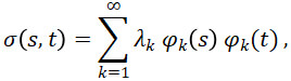
and the covariance function σ(s,t), which measures the covariance between any two points s and t within a function and can be estimated as
![]()
The methods we use are based on functional principal components analysis (FPCA), one of the key techniques in FDA because it provides an easily interpretable exploratory analysis of the data. FPCA relies on the assumption that functional data are independent and identically distributed (i.i.d.) random variables in the separable Hilbert space of square integrable functions on a bounded domain. In addition, FPCA assumes that the data are regularly and densely observed over the entire interval. Under the Hilbert space assumption and by Mercer’s Theorem, the covariance function can be written as
where λ_1≥λ_2≥⋯≥0 are the eigenvalues and φ_1, φ_2,… are the eigenfunctions of the covariance function. By the Karhunen-Loève Theorem, the FPCA expansion of function X_i (t) is
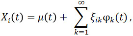
where μ(t) is the mean function and ![]() is the functional principal component, which is also called a score, associated with the kth eigenfunction
is the functional principal component, which is also called a score, associated with the kth eigenfunction ![]() . In order to compute or approximate this integral, dense and regularly observed functional data is necessary (Ramsay and Silverman, 2005; Yao et al, 2005).
. In order to compute or approximate this integral, dense and regularly observed functional data is necessary (Ramsay and Silverman, 2005; Yao et al, 2005).
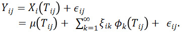
FPCA is traditionally computed under the assumptions that the data is regularly and densely observed over the entire bounded domain. However, real datasets often do not meet these assumptions. In order to perform FPCA when data do not meet these assumptions, we use the principal component analysis through conditional expectation (PACE) method. In this method, we estimate FPCA through conditional expectation on the observation times that we have data for. For sparse data, let ![]() be the jth observation of the random function
be the jth observation of the random function ![]() made at a random time
made at a random time ![]() , and let
, and let ![]() be the additional measurement errors that are assumed to be i.i.d. and independent of the random coefficients
be the additional measurement errors that are assumed to be i.i.d. and independent of the random coefficients ![]() , where i=1,…,n is the function number, j=1,…,Ni is the observation number within the ith function, and k=1,2,… is the number of the score in the FPCA expansion of
, where i=1,…,n is the function number, j=1,…,Ni is the observation number within the ith function, and k=1,2,… is the number of the score in the FPCA expansion of ![]() . The model is
. The model is
Let ![]() be a vector of all
be a vector of all ![]() values and
values and ![]() . The estimates for the FPCA scores are
. The estimates for the FPCA scores are
![]()
Using these estimates, the prediction for the trajectory ![]() , using the first Keigenfunctions, is
, using the first Keigenfunctions, is
![]() (Yao et al, 2005).
(Yao et al, 2005).
Overview of Methods for Functional Data of Multiple Variables
All of the methods described in Section 2.1 assume are for functional datasets describing one variable. When we have functional data with two or more variables, we have multivariate functional data. In multivariate functional datasets, each observation consists of p ≥2 functions X(1),…,X(p). They may be defined on different domains Τ1,…, Tp with possibly different dimensions. Each element X(j):Tj→R,j=1,…,p, is assumed to be in L2 (Tj), which is the space of real-valued square integrable functions defined in Tj, i.e.
![]() exists and is finite} (Staicu and Park, 2016).
exists and is finite} (Staicu and Park, 2016).
The p-dimensional tuple of functions can be written as
![]()
Like with univariate functional data, we can compute a mean function for multivariate functional data, which can be written as

Instead of a covariance function, which measures the covariance between any two points within a function, in multivariate functional data, we have a matrix of covariances which measures the covariance between any two points between the functions of any two variables. The matrix of covariances can be written as
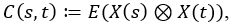
where ⊗ is the Kronecker product. The elementwise components of C(s,t) can be written as
![]()
Due to the assumption that each function X(j) is in L2(Tj ), for functions f=(f(1),…,f(p)), we can define the space H :=L2(Τ1 )×…×L2(Τp) and the inner product of two functions f and g
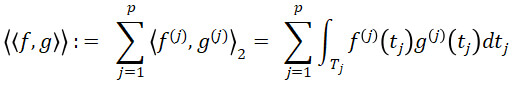
for f,g∈H. By Proposition 1 of (Happ and Greven, 2018), H is a Hilbert space with respect to the scalar product ⟨⟨⋅,⋅⟩⟩. To account for dependencies between variables, define the covariance operator Γ: H→H with the jth element of Γf ,f∈H given by
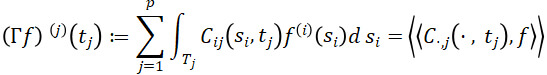
for tj∈Tj.
By Proposition 2 of (Happ and Greven, 2018), the covariance operator Γ is a linear, self-adjoint, and positive operator on H. By the Hilbert-Schmidt Theorem, it follows that there exists a complete orthonormal basis of eigenfunctions ψm∈ H, m∈N of Γ such that
Γψm=νmψm and νm→0 for m→∞.
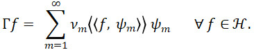
In particular, since Γ is a positive operator, it may be assumed without loss of generality (w.l.o.g.) that ν1≥ν2≥⋯≥0. Since the eigenfunctions ψm∈ H, m∈N form an orthonormal basis of H and Γ is self-adjoint, by the Spectral Theorem, it holds that
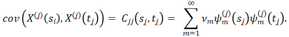
By the multivariate version of Mercer’s Theorem (Proposition 3 of (Happ and Greven, 2018)), for j=1,..,p and sj,tj∈Tj, it holds that
By the Multivariate Karhunen-Loève Theorem (Proposition 4 of (Happ and Greven, 2018)) under the assumptions of Proposition 2 of (Happ and Greven (2018)),
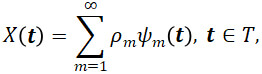
where the scores ρmψm are the inner product ⟨⟨X, ψm⟩⟩. Truncated Karhunen-Loève expansions, optimal M-dimensional approximations to X,
![]()
are often used in practice (Happ and Greven, 2018).
Multivariate FPCA
Given the finite Karhunen-Loève representation of multivariate functional data
a natural question is how this representation relates to the univariate Karhunen-Loève representations of each individual element of X(t). By Proposition 5 of (Happ and Greven (2018)), the multivariate functional vector X(t)=(X(1), …,X(p)) in ![]() has a finite Karhunen-Loève representation if and only if all univariate elements X(1), …,X(p) have a finite Karhunen-Loève representation. Assuming the univariate Karhunen-Loève representation
has a finite Karhunen-Loève representation if and only if all univariate elements X(1), …,X(p) have a finite Karhunen-Loève representation. Assuming the univariate Karhunen-Loève representation ![]() for each element X(j) of X, the positive eigenvalues ν1≥⋯≥νM>0 of Γ with
for each element X(j) of X, the positive eigenvalues ν1≥⋯≥νM>0 of Γ with ![]() correspond to the positive eigenvalues of the matrix
correspond to the positive eigenvalues of the matrix ![]() consisting of blocks
consisting of blocks ![]() with entries
with entries
![]()
for m=1,…,Mj, n=1,…,Mk, and j,k=1,…,p. These properties suggest a natural approach for estimating the MFPCA expansion of X(t) after calculating the univariate FPCAs for each individual element X(j). Given de-meaned samples x1,…,xN of X, we can estimate MFPCA in the following four steps:
- For each element X(j), estimate a univariate FPCA based on the observations
 ,…,
,…, . This results in estimate eigenfunctions
  and scores
  , i=1,…,N, m=1,…,Mj for suitably chosen truncation lags Mj. If the functional dataset available are sparse and irregularly sampled, the PACE method can be used to estimate the univariate FPCA for each element.
 - Define the matrix
 , where each row
  contains all estimated scores for a single observation. Compute the estimate of the block matrix Z, which consists of entries

as
- Compute the eigendecomposition of
 , which results in eigenvalues
  and orthonormal eigenvectors
  .
. - Estimates for the multivariate eigenfunctions are given by their elements
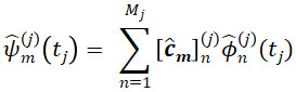
for tj∈Tj, and m=1,…,M+ and multivariate scores can be calculated via
![]() (Happ and Greven, 2018).
(Happ and Greven, 2018).
Implementation of Methods
We implement the methods described in Section 2 on three datasets:
- Statistical model simulated datasets
- Simulated ballistic missile trajectory dataset
- Northern California flight tracks dataset.
Each dataset has its own subsection of Section 3 that describes the dataset in greater detail and the results we get from implementing the methods. For all datasets, we implement the MFPCA and univariate FPCA (UFPCA) methods. (UFPCA is the same method as FPCA described in section 2.1. It is written as UFPCA in the implementation results to better distinguish it from MFPCA.) For UFPCA, this assumes that each variable is independent of one another, so we compute the FPCA expansion of each variable individually. For both MFPCA and UFPCA, the PACE method is used for computing the FPCA expansion of each individual variable.
For all three datasets, we originally observe full functions, To evaluate the effectiveness of the methods for sparsely and irregularly observed data, we compare the method results for the full dataset as well as medium (50-70% of the data missing) and high (80-90% of the data missing) sparsity levels. We sparsify the datasets according to the method described in (Yao et al, 2005) and implemented in the sparsify function, found in the R package funData (Happ-Kurz, 2020). Let minObs and maxObs be the minimum and maximum number of discrete observations in a function that are observed in a function, respectively. (For the medium sparsity settings, the minObs and maxObs values are 30% and 50% of the functional observation length, respectively. For the high sparsity case, the minObs and maxObs are 80% and 90% of the functional observational length, respectively.) For each element ![]() of an observed multivariate functional data object xi (the ith function in the jth feature), a random number
of an observed multivariate functional data object xi (the ith function in the jth feature), a random number ![]() ∈{minObs,maxObs} of observation points is generated. The points are sampled uniformly from the full grid {tj,1,…,tj,Sj⊂Tj, resulting in observations
∈{minObs,maxObs} of observation points is generated. The points are sampled uniformly from the full grid {tj,1,…,tj,Sj⊂Tj, resulting in observations

For the statistical model simulated datasets, we will compare the method results when there is or is no measurement error. Since we don’t have any information about the measurement error in the simulated ballistic missile trajectory and Northern California flight tracks datasets, we do not evaluate our results in the context of measurement error for these two datasets.
To evaluate the method results, the quantitative metric we use is the mean relative squared error (MRSE),
![]()
which measures the relative error between the estimated and actual functions. We evaluate our results taking into account as many of the following properties as possible for each dataset. For each property, we list all possible settings.
- Method: how does taking into account dependencies between covariates affect these estimation results?
- Possible settings: MFPCA and UFPCA
- Variability between functions: how much variability and diversity between functions exist in the dataset? This can be an indication of how much the dataset deviates from the usual i.i.d. assumption made in FDA methods. This property is evaluated for the statistical model simulated datasets and Northern California flight tracks data only, as the simulated ballistic missile dataset contains very uniform data.
- Possible settings depend on each dataset
- Data sparsity: what percentage of the data is observed?
- Possible settings: full data, medium sparsity, and high sparsity.
- Measurement error: is the data perfectly observed, or are there measurement errors in the data? This property is evaluated for the statistical model simulated datasets only, as this is the only dataset where we have information available on measurement error.
a. Possible settings: no measurement error and with measurement error
We expect that estimation error will increase as any or all of the three properties above increase. Currently, there are no theoretical mathematical developments comparing the estimation performance between MFPCA and UFPCA. All possible combinations of settings of examined properties define the cases examined in each forthcoming dataset.
All statistical model simulated datasets are generated and all data analyses are conducted utilizing the MFPCA and funData packages in the R programming language (Happ and Greven, 2018; Happ-Kurz, 2020).
Statistical model simulated datasets
After defining various settings that have differing levels of variability between trajectories, sparsity, and measurement error, for each setting, we simulate 100 datasets with N=200 observations from the MFPCA model
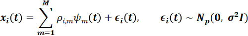
for t∈Τ, i=1,…,N, and where the mean function μ(t)=0.
We utilize two sets of basis functions to generate our data. We simulate data from the first eight Fourier basis functions on [0, 1] and the first eight Wiener basis functions on [0, 1]. They are each split into p=2 parts, which means there are two elements to each observation xi(t). Plots of the basis functions used are in Figure 1.
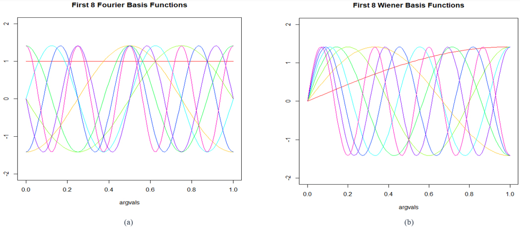
Figure 1. Plots of the first eight Fourier basis functions (a) and first eight Wiener basis functions (b) on [0, 1].
For the data generated from the first eight Fourier basis functions, the scores ![]() are independent samples from a
are independent samples from a ![]() distribution for eigenvalues with linear
distribution for eigenvalues with linear ![]() decrease. For the data generated from the first eight Wiener basis functions, the scores are independent samples from
decrease. For the data generated from the first eight Wiener basis functions, the scores are independent samples from ![]() for eigenvalues with exponential
for eigenvalues with exponential ![]() decrease (Happ and Greven, 2018).
decrease (Happ and Greven, 2018).
In order to account for the amount of variability between functions in a dataset, we construct the following four datasets. The list starts with the names given to the datasets.
- Fourier: 200 functional observations generated from the first eight Fourier basis functions
- Fourier + Wiener:100 functional observations generated from the first eight Fourier basis functions and 100 functional observations generated from the first eight Wiener basis functions
- Fourier + Wiener x 10:100 functional observations generated from the first eight Fourier basis functions and 100 functional observations generated from the first eight Wiener basis functions, with the observations from the Wiener basis functions multiplied by 10
- Fourier + Wiener x 100:100 functional observations generated from the first eight Fourier basis functions and 100 functional observations generated from the first eight Wiener basis functions, with the observations from the Wiener basis functions multiplied by 100
We increase the variability between functions by including functions generated from two different set of basis functions, Fourier and Wiener. By multiplying the Wiener generated functions by 10, and then by 100, we further increase the variability between functions.
Plots of one simulation of functional observations for each of the above four dataset can be found in Figure 2. For each observation, since there are two elements, we plot each element, denoted as x1 and x2, versus t.
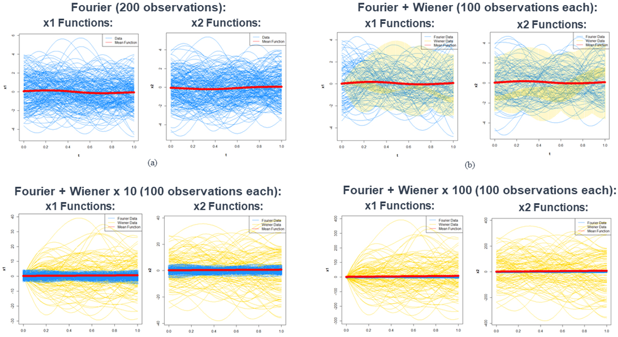
Figure 2. Plots of functional data generated in one simulated dataset consisting of the four statistical model simulated datasets (Fourier, Fourier + Wiener, Fourier + Wiener x 10, and Fourier + Wiener x 100), which are ordered (a)-(d). For all plots, data generated from the Fourier basis functions are colored blue, and data generated from the Wiener basis functions are colored green, the mean function of the data is the thick red line.
For all datasets, we consider data without (σ2=0) and with measurement error (σ2=0.25). When we consider the full data and medium sparsity settings, the MFPCA is based on M1=M2=8 univariate functional principal components that are calculated by the PACE algorithm. When we consider the high sparsity setting, the MFPCA is based on M1=M2=5 univariate functional principal components to make computing the univariate FPCA feasible.
For each of our four datasets, we compute the average MRSE values of the estimation results over 100 datasets for all 12 possible combinations of estimation methods and the dataset properties of sparsity and presence of measurement error. Table 2 contains the average MRSE values for all four datasets and all 12 combinations of settings. These results are contained in the last 12 columns of Table 2, which are listed as columns (a)-(l). We further analyze the results in the context of variability between functions, data sparsity, measurement error, and method. Holding all of the settings for the other three properties the same, we examine each of the four properties and its effect on the average MRSE values.
Table 2. Average MRSE values for all statistical simulation datasets and all dataset properties combinations.
| Dataset | (a) Full Data, No Measure-ment Error, MFPCA |
(b) Full Data, No Measure-ment Error, UFPCA |
(c) Full Data, With Measure-ment Error, MFPCA |
(d) Full Data, With Measure-ment Error, UFPCA |
(e) Medium Sparsity, No Measure-ment Error, MFPCA |
(f) Medium Sparsity, No Measure-ment Error, UFPCA |
(g) Medium Sparsity, With Measure-ment Error, MFPCA |
(h) Medium Sparsity, With Measure-ment Error, UFPCA |
(i) High Sparsity, No Measure-ment Error, MFPCA |
(j) High Sparsity, No Measure-ment Error, UFPCA |
(k) High Sparsity, With Measure-ment Error, MFPCA |
(l) High Sparsity, With Measure-ment Error, UFPCA |
| Fourier | 0.00284 | 0.002821 | 0.126228 | 0.125008 | 0.005749 | 0.005884 | 0.023072 | 0.027001 | 0.468063 | 0.051878 | 0.472821 | 0.136443 |
| Fourier + Wiener (100 observa- tions each) |
0.025695 | 0.003217 | 0.188 | 0.169513 | 0.028455 | 0.006379 | 0.05044 | 0.038547 | 0.427267 | 0.068913 | 0.429469 | 0.124431 |
| Fourier + Wiener x 10 (100 observa- tions each) |
0.045145 | 0.030446 | 0.102414 | 0.08907 | 0.052675 | 0.034494 | 0.061559 | 0.044444 | 0.452839 | 0.136372 | 0.474834 | 0.202709 |
| Fourier + Wiener x 100 (100 observa- tions each) |
0.093695 | 0.068702 | 0.141213 | 0.119127 | 0.202036 | 0.125201 | 0.210061 | 0.13446 | 3.173803 | 0.889492 | 3.259918 | 1.051794 |
Variability Between Functions
The effect of variability between functions can be seen by comparing results between the four datasets along any one column in Table 2. The four datasets we generate are designed to increase in variability between functions, so as we go from top to bottom in any column, we expect the average MRSE values to increase. The expected results are found in columns (a)-(b), (e)-(h) (all of the medium sparsity settings), (j), and (k). However, the expected results are not found in the remaining columns.In columns (c) and (d), which represents the cases of full data with measurement error, the dataset with 100 observations of Fourier generated functions and 100 observations of Wiener observations multiplied by 10 has lower average MRSE values than the datasets with 200 Fourier generated observations and 100 each of Fourier and Wiener generated observations. For UFPCA (column (d)), the dataset with 100 Fourier observations and 100 Wiener observations multiplied by 100 has lower average MRSE values than the than the datasets with 200 Fourier generated observations and 100 each of Fourier and Wiener generated observations.
In columns (i) and (l), which represent two high sparsity cases, the dataset with 100 observations each from the Fourier and Wiener basis functions has lower average MRSE values than the dataset with 200 Fourier generated observations. In column (i), the dataset with 100 Fourier observations and 100 Wiener observations multiplied by 10 has lower average MRSE values than the dataset with 200 Fourier observations.
We also note that in the medium and high sparsity cases, the magnitude of increase in average MRSE values (compared with the other datasets) for the dataset with 100 Fourier observations and 100 Wiener observations multiplied by 100 is noticeably higher as sparsity increases.
Method
The effect of the method used for estimating the function is assessed by comparing the values in one row over a pair of columns where the sparsity and measurement error settings are the same. For example, we compare columns (a) and (b) in the first row, which are both for the settings of full data and no measurement error for the dataset with 200 Fourier observations. The only difference between the two columns is the estimation method. For most cases where UFPCA has lower average MRSE values than MFPCA. The exceptions are for the medium sparsity cases of the dataset with 200 Fourier observations (row one, columns (e) & (f) and columns (g) and (h)). In these pairings, MFPCA has lower average MRSE values than UFPCA.
We also note that in the high sparsity cases (columns (k) and (l)), we find that UFPCA has much lower average MRSE values than MFPCA, by a much higher magnitude than is observed in the full data and medium sparsity cases.
Data Sparsity
The effect of data sparsity is assessed by comparing the set of three columns (in one row for the same dataset) where the settings of measurement error and method are the same. For example, comparing columns (a), (e), and (i) lets us see the effects of sparsity for the cases where there is no measurement error and the MFPCA method is used to estimate functions. For all datasets, and for all settings of measurement error and method, we find that increased sparsity results in increased average MRSE values.
Measurement Error
The effect of measurement error by comparing the set of two columns (in one row for the same dataset), where the settings of sparsity and method are the same. For example, comparing columns (a) and (c) lets us see the effects of measurement error for the cases where there is full data and the MFPCA method is used to estimate functions. For all datasets, and for all settings of sparsity and method, we find that the presence of measurement error results in increased average MRSE values. In some high sparsity cases, such as seen in columns (i) and (k), the presence of measurement error only results in small increases in average MRSE values. This may serve as empirical evidence that the PACE method is a robust method for estimating FPCA quantities in the presence of measurement error.
Simulated ballistic missile trajectory dataset
The simulated ballistic missile trajectory dataset is a set of 500 trajectories that are generated by a physics model that notionally propagates objects according to a path of a ballistic missile. The dataset consists of 200 discretely observed points for each trajectory. In order to have all 500 trajectories on the same bounded interval, we standardize the trajectory times to the interval [0, 1], so the trajectory times are the “percent progress of the trajectory.” The six covariates in our dataset are the X, Y, and Z positions and velocities of the trajectory relative to the center of the Earth. These covariates are in the Earth-Center Earth-Fixed (ECEF) coordinate system.Figure 3 shows the plots of the XYZ positions and velocity versus the percent progress of trajectory. These plots tell us that the trajectories in this dataset are very uniform and very closely match the i.i.d. assumption typically made in FDA methods.
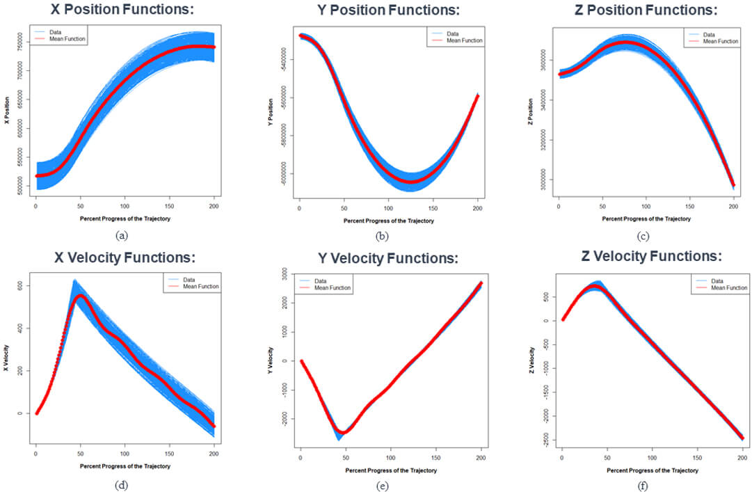
Figure 3. Plots of the XYZ positions and velocities versus the percent progress of trajectory for all trajectories in the simulated ballistic missile trajectory dataset. The trajectories are represented as blue lines. The red lines are the mean functions of each covariate.
Since we have only one dataset, we don’t have multiple measures of variability between functions. We also don’t have any information on the measurement error with this dataset. Therefore, we compute the MRSE values for all six possible combinations of data sparsity and method. Table 3 shows the MRSE values for all six possible combinations of sparsity and method. These results are listed in columns (a)-(f) of Table 3. We further analyze the results in the context of sparsity and method.
Table 3. MRSE values for simulated ballistic missile trajectory dataset and all dataset properties combinations.
| (a) FullData, MFPCA |
(b) FullData, UFPCA |
(c) Medium Sparsity, MFPCA |
(d) Medium Sparsity, UFPCA |
(e) High Sparsity, MFPCA |
(f) High Sparsity, UFPCA |
| 7.35118 x 10⁻⁸ | 7.11116 x 10⁻⁸ | 8.11026 x 10⁻⁸ | 8.00473 x 10⁻⁸ | 7.72053 x 10⁻⁸ | 8.02807 x 10⁻⁸ |
Data Sparsity – For UFPCA (columns (b), (d), and (f)), MRSE values increase as data sparsity increases. However, for MFPCA (columns (a), (c), and (e)), high sparsity has a lower MRSE value than medium sparsity. In the case of MFPCA, this may indicate that even though in the high sparsity case, a smaller amount of the data is observed, the data that was observed in the high sparsity case is more useful in obtaining more accurate estimates of the actual trajectories.
Method – For high sparsity (columns (e) and (f)), MFPCA has a lower MRSE value than UFPCA. However, for both full data (columns (a) and (b)) and medium sparsity (columns (c) and (d)), UFPCA’s MRSE values are lower than that of MFPCA.
Northern California flight tracks dataset
The publicly available dataset consists of radar tracks in terminal radar approach control (TRACON). The dataset contains flight tracks over the San Francisco Bay area for the first three months of 2006. The records cover the Northern California TRACON (NCT), which is a cylinder of radius 80 kilometers and height 6,000 meters centered at Oakland International Airport (OAK). The NCT contains three main commercial airports, the Oakland, San Francisco (SFO), and San Jose (SJC) International Airports, as well as many smaller airports. The NCT is the fourth busiest terminal area in the U.S. with an average of 133,000 flight instrument operations per month in 2006. The data, which are made of the position and speed of aircraft, are organized by flight and contain metadata for each flight, which include the type of operation (departure/arrival), origin and destination airports, aircraft type (business, jet, helicopter, other, etc.), date and time of the beginning of record, duration of the record, etc. (“Flight tracks, Northern California TRACON.”; Gariel et al, 2011).
For our analyses, we focus on 423 tracks of flights originating from San Jose International Airport (we refer to this airport by its airport code SJC from now on) and a random sample of 10,000 flights originating from San Francisco International Airport (we refer to this airport by its airport code SFO from now on). For each track, our four covariates are the XYZ positions (relative to OAK, the center of the NCT) and velocity. For all tracks, we interpolate the trajectories to 101 points in the interval [0, 1], so our continuum variable is “percent progress of the trajectory.”
To assess the effects of different levels of diversity in tracks, and thus, variability between functions, we set up the following four datasets:
- SFO Origin Tracks: the 10,000 flight tracks originating from SFO
- SJC Origin Tracks: the 423 flight tracks originating from SJC
- SFO + SJC Origin Tracks (423 Tracks Each): a balanced dataset with the 423 flight tracks originating from SJC and a random selection of 423 track out of the 10,000 SFO origin tracks
- SFO (10,000) + SJC (423) Origin Tracks: contains all 10,000 flight tracks originating from SFO and all 423 flight tracks originating from SJC
Figure 4 shows plots of the data for each of the above four datasets. For each dataset, we make the following three plots:
- Plot of the flight tracks in the XY plane, including the beginning and end points of the tracks
- Plot of X position vs. percent progress of trajectory for all tracks, along with the mean function of X position in the dataset
- Plot of Y position vs. percent progress of trajectory for all tracks, along with the mean function of Y position in the dataset
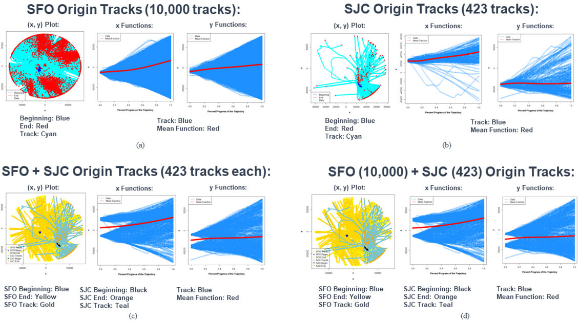
Figure 4. Plots of the XY positions, along with the beginning and end points, of the flight tracks; X position vs. percent progress of trajectory; and Y position vs. percent progress of trajectory for the four smaller datasets created out of the Northern California TRACON flight tracks dataset. In the XY positions plots, the colors of the tracks, beginning, and end points for the SFO and SJC origin tracks are given below those plots. For the X position and Y position vs. percent progress of trajectory plots, the tracks are plotted in blue, and the mean functions are plotted in red.
The XY positions plot of the SFO origin tracks show that flights can go in any direction after departing from SFO, but the highest concentration of flights travel north, northeast, and south from SFO. On the other hand, the XY positions plot of the SJC origin tracks show that not as many flights departing from SJC travel in a westerly direction. Most of the flight tracks go north, south, or east of SJC. The XY position plots for the dataset with all SFO and SJC origin tracks covers all possible directions, while the dataset with 423 tracks from each airport has some directions where we don’t observe flights flying to. Therefore, the order of the four datasets by variability between functions is as listed above.
Since we do not have any information about measurement error for the radar system collecting the flight tracks data, we do not consider the effects of measurement error. For each of our four datasets, we compute the MRSE values of the estimation results for all six possible combinations of estimation methods and sparsity. Table 4 shows MRSE values for all six possible combinations of sparsity and method over our four datasets. These results are listed in columns (a)-(f) of Table 4. We further analyze the results in the context of variability between functions, sparsity, and method.
Table 4. MRSE values for Northern California TRACON flight tracks datasets and all dataset properties combinations.
| Dataset | (a) FullData, MFPCA |
(b) FullData, UFPCA |
(c) Medium Sparsity, MFPCA |
(d) Medium Sparsity, UFPCA |
(e) High Sparsity, MFPCA |
(f) High Sparsity, UFPCA |
| SFO Origin Tracks (10,000 Tracks) | 0.005033 | 0.004984 | 0.00525 | 1.051036 | 0.006379 | 1.051732 |
| SJC Origin Tracks (423 Tracks) | 0.001398 | 0.000697 | 0.001481 | 1.167057 | 0.001984 | 1.166021 |
| SFO + SJC Origin Tracks (423 Tracks Each) | 0.006498 | 0.006092 | 0.004529 | 1.10268 | 0.00704 | 1.10765 |
| SFO (10,000 Tracks) + SJC (423 Tracks) Origin Tracks | 0.005819 | 0.005143 | 0.00607 | 1.05447 | 0.00522 | 1.055745 |
Variability Between Functions – We expect the MRSE value for the SFO origin tracks dataset to be higher than that of the SJC origin tracks dataset. That holds true, except for the cases of medium sparsity and MFPCA method (column (c)) and high sparsity and UFPCA method (column (f)). We also expect the MRSE values for the dataset with 423 tracks each originating from SFO and SJC to be lower than the MRSE values for the dataset with all 10,000 SFO origin tracks and 423 SJC origin tracks. However, we find that only holds for the case of medium sparsity and MFPCA method (column (c)). For all other cases, the dataset with all 10,000 SFO origin tracks and 423 SJC origin tracks has lower MRSE values than the dataset with 423 tracks each originating from SFO and SJC. With the exception of the case of medium sparsity and MFPCA method (column (c)), the MRSE values for the dataset with 423 tracks each originating from SFO and SJC are higher than the MRSE values for the dataset with 10,000 SFO origin tracks. With the exception of the case of high sparsity and MFPCA method (column (e)), the MRSE values for the dataset with all 10,000 SFO origin tracks and 423 SJC origin tracks are higher than the MRSE values for the SFO origin tracks dataset. The expected trends in MRSE values with respect to variability between functions do not hold true in all cases.
Data Sparsity – In most cases, increased data sparsity results in increased MRSE values. However, there are two notable exceptions. First, when applying UFPCA to the SJC origin tracks dataset, there is a decrease in MRSE when we go from medium to high sparsity (row 2, columns (d) and (f)). Second, when applying MFPCA to the dataset with 423 tracks each originating from SFO and SJC, MRSE decreases when we go from hill data to medium sparsity (row 3, columns (a) and (c)). In these two exceptions, this may indicate that even though there is a reduction in the amount of data available, the actual observed data in the more sparse datasets are more valuable to obtaining more accurate estimates of the flight tracks.
Method – For full data (columns (a) and (b)), UFPCA has lower MRSE values than MFPCA. However, for both medium sparsity (columns (c) and (d)) and high sparsity (columns (e) and (f)), MFPCA has lower MRSE values than UFPCA. These findings hold true for all four datasets.
Overall Findings
In our implementation results, we expect that increases in variability between functions, data sparsity, and measurement error all correlate with increases in estimation error (the MRSE values). For the methods, MFPCA and UFPCA, we expect that accounting for dependencies between covariates has an effect on the MRSE values, but there is currently no rigorous theory on the nature of these effects. Throughout the results for our three types of datasets, our expected trends with respect to variability between functions, data sparsity, and measurement error hold true in many cases, but not always. In the statistical model simulated datasets, the presence of measurement error increases the MRSE values, and the increase in MRSE values are smaller in high sparsity datasets. This may be empirical evidence that when we have lower amounts of observed data, the measurement error does not accumulate as much, which does not have as great of a detrimental effect on estimation performance. In addition, this may also show the robustness of the PACE method with computing FPCA expansions in the presence of sparsity. However, for the factors of method, variability between functions, and data sparsity, we see cases win unexpected outcomes. There are likely dependencies between the methods, variability between functions, data sparsity, and measurement error that contribute to estimation error. The nature of these dependences may be such that holding everything else constant will not allow us to pinpoint the full nature of the contributions of any one data property of estimation error. This necessitates the need for further study into the dependencies between data properties. There may also be other contributors to estimation error besides these four factors.
Conclusion
We present methods for estimating entire multivariate functional data observations when the observed data available is sparsely and irregularly observed and contains measurement error. This represents a departure from most FDA methods, which assume that observed data is densely and regularly observed over the bounded domain, and if the data contains multiple variables, they are independent of one another. We use the PACE method to estimate FPCA expansions for functions that are sparsely and irregularly observed with measurement error. The MFPCA method, when utilizing the PACE method to compute the FPCA expansion for each variable, can reconstruct entire multivariate functions.We implement the MFPCA and UFPCA methods on three types of datasets (statistical model simulated, simulated ballistic missile trajectory, and Northern California TRACON flight tracks) to empirically assess the performance of these methods in the context of the method used, variability between functions, data sparsity, and measurement error. While we expect accounting for dependencies between covariates to have an effect on estimation error, there is currently no rigorous theory on that effect, so it is difficult to know what to expect. Throughout our implementation results, while we see many cases where increases in variability between functions, data sparsity, and measurement error results in greater estimation error, this does not always hold true. Therefore, much of the future work we suggest is geared towards the goal of understanding why in a rigorous manner.
Future Work
The first area of future work is better defining and utilizing the covariance between covariates for functional data. The covariance function measures pairwise covariances between any two points on a single function. The covariate operator in multivariate functional data sums up all of the pairwise covariance matrices between any two variables, which may mask individual pairwise covariances between variables that are more significant than others. Further, the current statistical model simulations of multivariate functional data does not explicitly account for the covariance between variables. In MFPCA estimation, any dependencies between variables is only accounted for when taking the eigendecomposition of the block matrix consisting of the scores from the FPCA expansion of each individual covariate’s functions. The covariance operator is not utilized in MFPCA estimation. Better characterization and utilization of the dependencies between covariates in functional data will allow better assessment of the effects of dependencies between covariates on any functional data analysis task, including reconstruction of partially observed multivariate functions.The second area of future work is developing a quantitative metric that measures variability between functions as a whole. Functional variance processes (Müller et al, 2006), the current measure widely used to measure variability in functional data, measures variance in functional data with respect to the continuum variable t. However, this does not provide a measure of the overall variance between functions, regardless of the value of t. Successful development of this metric can provide a more objective measure of variability and better assessment of the relationship between variability between functions and functional data analysis results.
The third area of future work is developing the notion of a probability density function for functional data. It is argued in (Delaigle and Hall, 2010) it is not possible to derive a probability density function for functional data. Even if it is not possible to develop a “traditional” statistical notion of a probability density function for functional data, successfully developing a notion of a probability density function, in which a stated equation can deterministically characterize the statistical properties of a functional dataset, would greatly aid in many open FDA problems regarding the statistical properties of functional data. Examples include defining whether a function is in-distribution or out-of-distribution of a trained FDA model, defining variability between functions, helping to clarify the concept of i.i.d. in functional data, and developing the theoretical properties that can help explain the estimation performances of the MFPCA and UFPCA methods.
The fourth area of future work is characterizing the value of information of specific snippets or points within functions with respect to functional data analysis results. In our implementation results, we see a number of instances where estimation error decreases as data sparsity increases. This can be an indication that even if a function is irregularly and sparsely observed, if the right portions of the function are observed that provide the most important behaviors of the function, that function can be reconstructed well. Extending to any functional data analysis task involving sparsely and irregularly observed functions, being able to characterize the value of information of any segment or even individual points of a function that can capture critical information about the function can greatly help in ensuring that the critical functional data points or snippets are observed.
The development of the multivariate extensions of the confidence bands for individual trajectories and the Akaike Information Criterion (AIC) for estimating the appropriate number of eigenfunctions in the MFPCA estimations developed in (Yao et al, 2005) can provide insights into the value of information for the currently available data. The confidence bands can reveal the uncertainty in the estimates of the complete trajectories in relation to the available data. The AIC results can also help determine if the counterintuitive results we observe in our data analyses are sensitive to the number of eigenfunctions used in the FPCA representations for each feature. The value of information metric would provide a quantitative assessment of the information contained in a specific point or functional snippet with respect to the entire function, which would be correlated to the performance of estimating the entire function.
The fifth area of future work is characterizing the dependencies between the estimation methods, variability between functions, data sparsity, and measurement error, and how these dependencies affect estimation error. The data properties (variability between functions, data sparsity, and measurement error) are all dependent with one another because they describe the same dataset. Determining the nature of these dependencies may require other measures than the commonly-used covariance, which measures linear dependencies between two variables. There may be non-linear dependencies between these properties. Successful characterization of the dependencies between these data properties can not only help attribute estimation error to specific properties, it can also help further understand how the relationship between data properties affect estimation performance with specific methods like MFPCA and UFPCA.
Rigorous characterization of the properties of functional data allow analysts to better understand the properties of functional datasets through more objective, quantitative metrics. This promotes better understanding of differences between datasets, analyses, and deciding on various settings to compare. This has great relevance to both data analysts and systems engineers who make decisions on the specific methods and strategies used in an analysis pipeline.
Acknowledgements
We are very grateful to Josey Stevens for generating the unclassified ballistic missile trajectories dataset, and for the financial support of the Missile Defense Agency (MDA) and the Janney Grants program at the Johns Hopkins University Applied Physics Laboratory.
References
Benko, Michal, 2006. Functional Data Analysis with Applications in Finance. Ph.D. dissertation, Humboldt University of Berlin.
Delaigle, Aurore and Peter Hall, 2010. Defining probability density for a distribution of random functions. The Annals of Statistics 38 (2): 1171-1193.
“Flight tracks, Northern California TRACON.” https://catalog.data.gov/dataset/flight- tracks-northern-california-tracon.
Gariel, Maxime, Ashok Shristava, and Eric Feron, 2011. Trajectory Clustering and an Application to Airspace Monitoring. IEEE Transactions on Intelligent Transportation Systems 12 (4): 1511-1524.
Happ, Clara and Sonja Greven, 2018. Multivariate Functional Principal Component Analysis for Data Observed on Different (Dimensional) Domains. Journal of the American Statistical Association 113: 649-659.
Happ-Kurz, Clara, 2020. Object-Oriented Software for Functional Data. Journal of Statistical Software 93(5): 1-38.
Mishra, Vinod K. and Bhikhari Tharu, 2021. Functional Data Analysis of the RT Tactical Data. Technical Report, DEVCOM Army Research Laboratory.
Müller, Hans-Georg, Rituparna Sen, and Ulrich Stadtmüller, 2011. Functional Data Analysis for Volatility. Journal of Econometrics, 165 (2): 233-245.
Müller, Hans-Georg, Ulrich Stadtmüller, and Fang Yao, 2006. Functional Variance Processes. Journal of the American Statistical Association, 101:475: 1007-1018.
Ramsay, James O. and Bernard W. Silverman, 2005. Functional Data Analysis, second ed. New York: Springer Series in Statistics.
Shangguan, Pengpeng, Taorong Qiu, Tao Liu, Shuli Zou, Zhou Liu, and Siwei Zhang, 2020. Feature extraction of EEG signals based on functional data analysis and its application to recognition of driver fatigue state. Physiological Measurement, 41 (12):
Staicu, Ana-Maria and So Young Park. “Short Course on Applied Functional Data Analysis.” Department of Mathematics and Computer Science, University Babes Bolyai. May 23-27, 2.16.
Tian, Tian S., 2010. Functional Data Analysis in Brain Imaging Studies. Frontiers in Psychology, 1:35: 1-11.
Vinue, Guillermo and Irene Epifanio, 2019. Forecasting basketball players’ performance using sparse functional data. Statistical Analysis and Data Mining: The ASA Data Science Journal, 12 (6): 1864-1932.
Wakim, Alexander and Jimmy Jin, 2014. Functional Data Analysis of Aging Curves in Sports. arXiv.
Wang, Jane-Ling, Jeng-Min Chiou, and Hans-Georg Müller, 2015. Review of functional data analysis. Annual Review of Statistics and Its Application, 3 (1): 257-295.
Yao, Fang, Hans-Georg Müller, and Jane-Ling Wang, 2005. Functional data analysis for sparse longitudinal data. Journal of the American Statistical Association, 100: 577-590.
Author Biographies
Dr. Maximillian G. Chen is a Senior Professional Staff member at the Johns Hopkins University Applied Physics Laboratory (JHUAPL). He is interested in developing novel statistical methodologies in the areas of high-dimensional data analysis, dimension reduction and hypothesis testing methods for matrix- and tensor-variate data, functional data analysis, dependent data analysis, and data-driven uncertainty quantification. He is a member of the American Statistical Association. Dr. Chen holds B.S. degrees in Accounting and Mathematics from the University of Maryland, College Park, and M.S. and Ph.D. degrees in Statistics from Cornell University.