Aerial refueling (AR) is the process of using an apparatus to pass aviation fuel from one aircraft (acting as a tanker) to another (acting as a receiver) in flight. The AR mission is usually conducted to increase the range or endurance of military receiver aircraft, be it for combat, transport, or reconnaissance. While it is not required, many world militaries employ purpose-built tanker aircraft to fulfill this mission. One of many technical requirements for AR is the tanker’s ability to pass fuel from the tanker to the receiver at a near constant pressure within safety limits while maximizing efficiency.

The study of fuel pressure behaviors is a key component of the test and evaluation (T&E) of new tanker/receiver aircraft pairings. During AR operations, fuel from a tanker is transferred through various lengths and diameters of pipes and hoses into multiple individual fuel tanks in the receiver aircraft. Valves within the receiver aircraft’s fuel system open and close throughout the fuel transfer process to direct fuel to the various tanks and maintain aircraft balance until capacity is reached. As the valves open and close, the fuel flow rate from the tanker is disrupted and the pressure in the combined fuel system becomes variable. In turn, the tanker fuel delivery system must constantly adjust the pressure at which it provides fuel to maintain safe operations. Over time, patterns or behaviors in fuel pressure can emerge, such as spikes, drops, oscillations, and steady states. Fuel pressure data streams are therefore evaluated based on established criterion over a range of starting and ending receiver fuel weights to confirm that safe pressure levels are maintained throughout the fuel transfer process. Military specifications and references for AR may be found in MIL-HDBK-516C (sec 8.7.1.7-8), ATP 3.3.4.5 Edition B (sec 1.12.1-2), and ATP 3.3.4.6 Edition A (sec 2.5-7).

In practice, it can be difficult for AR engineers to identify individual fuel pressure behaviors within a data stream because some of the various behaviors can occur simultaneously and are highly polymorphic (a behavior type may look different from one occurrence to the next). While individual instances of pressure exceedance can be easily identified, the underlying and more nuanced fuel pressure behaviors can be difficult to consistently identify and differentiate across the varied experience levels of the AR engineers performing the data analysis at any given time. Additionally, reporting time constraints and resource limitations have precluded the engineers from routinely performing more detailed analyses and developing an authoritative consensus. As a result, an authoritative truth source for fuel pressure behavior labels does not exist for any given dataset. This paper details how the AR engineers collaborated with statisticians and data scientists to develop a defensible, reproducible, and consistent method to identify and classify various fuel pressure behaviors.

Classifying fuel pressure behavior using statistical or machine learning methods may seem deceptively simple in this context. At first glance, one might employ a supervised classification model (machine learning-based or otherwise) which would be trained on SME-labeled data that exhibit the various problematic behavior. However, any proposed solution must overcome several non-trivial challenges. 

The first challenge was that, while most of the problematic fuel pressure behaviors may seem simple to identify, each behavior is highly polymorphic, and some behaviors can occur simultaneously. For our purposes, polymorphism refers to the property that any given occurrence of a particular behavior type will usually not be identical to any other occurrence due to the unique combination of stochastic and deterministic physical processes involved (e.g., atmospheric conditions, valve position, pump setting, remaining receiver capacity). Rather, behavior types are distinguished by certain characteristics like the range in fuel pressure between adjacent troughs and crests, the magnitude of individual troughs and crests in relation to defined thresholds, and duration of behavior. A multivariate classification model (or multiple univariate classification models) would need to be trained on a wide variety of data-stream cases across multiple tankers and receivers to be capable of adequate predictive accuracy. 

The second challenge is that the required correctly labeled data does not exist because of SME time constraints and the difficulty of consistently and defensibly classifying fuel pressure behaviors across tankers, receivers, and AR engineers. Imperfectly labeled data constitute a form of measurement error that would lead to additional prediction error from any trained model. 

A third challenge came to light after we began to build a model: the types of fuel pressure behaviors of interest had not been well characterized and canonized prior to this modeling effort, partially due to the polymorphic nature of each behavior type. The process of iteratively building a model was powerful in eliciting information about additional behavior types, definition nuances, and edge cases from the SMEs. We determined that characterizing and officially defining the fuel pressure behavior types, refining the definitions over time, and building an expert system (ES) AI based on the behavior definitions would be the easiest way to overcome these challenges and produce a viable automatic classification system.

An expert system (ES) is a form of artificial intelligence that was first invented in the mid to -late 1970’s before becoming widely used in the 1980’s and beyond (Aronson, 2003). An ES is so named because it is designed to incorporate and apply the domain-specific knowledge of an expert to complete set tasks. For example, expert systems were originally envisioned to provide analytical services about subjects like logistics (XCON; Leonard-Barton & Sviokla, 1988), accounting (ExperTAX; Leonard-Barton & Sviokla, 1988), geology (MUDMAN; Leonard-Barton & Sviokla, 1988), chemistry (Dendral; Leonard-Barton & Sviokla, 1988), and medicine (MYCIN; Copeland, 2018; Shortliffe, 1977). At its core, an ES contains a corpus of knowledge, well-defined definitions, and logical rules that can automatically identify patterns or complete tasks. Developers use a process called knowledge discovery or knowledge engineering to elicit information and rules from SMEs and incorporate that body of knowledge into a program that completes specific expert tasks. Many situations where ES have previously been used, or where ES had partially solved a problem have since been addressed using deep learning models (e.g., speech to text transcription and translating between languages; Hayes-Roth, Waterman, & Lenat, 1983). However, the general tools and principles of ES are still used and are so commonplace that an ES is often not recognized as a form of AI by the layman.

We have pursued fuel pressure behavior classification via ES because 1) fuel pressure behaviors have discernable characteristics, 2) the classification work has historically been done by SMEs and AR engineers that relied on engineering judgment, and 3) no definitive truth source exists for any given fuel pressure time series. Importantly, applying an ES to fuel pressure behavior classification entails an implicit task of sub-dividing the data stream into segments of adjacent data points that have similar characteristics. Sub-dividing the data stream allows an ES to apply rules that identify the beginning and end of each behavior. Changepoint detection algorithms are a natural choice to complete this sub-division task.

A changepoint can be viewed as a natural breakpoint between two segments (where each segment consists of at least two observations) of a time series data stream where the underlying process that produces the data has changed in some discernable way. Changepoint detection algorithms or models can use various parametric or non-parametric methods to estimate the location of these natural changes. Identifying changepoints effectively separates or clusters the data into segments of adjacent observations that have common characteristics. Changepoint detection algorithms may be considered an unsupervised form of machine learning because the data do not already contain markers or labels for where the underlying process changed (Aminikhanghahi & Cook, 2017). These algorithms have a wide range of applications, from medical condition monitoring and speech recognition (Aminikhanghahi & Cook, 2017), to manufacturing process control (Wu, Li, Lanye Hu, & Hu, 2022), and other forms of anomaly detection.

The remainder of the paper will proceed as follows: first, we introduce our changepoint detection algorithm of choice, discuss the algorithm’s properties, and discuss how we implement it on a fuel pressure data stream. Second, we explain the expert system AI that we produced, explain the types of behavior that the system identifies, and introduce metrics that quantify the output of the AI. Third, we discuss the T&E process for the entire FACS system. We then present real data examples where the FACS system was applied and discuss the implications on T&E for aerial refueling platforms.

The changepoint detection method that we employ in this paper is the Pruned Exact Linear Time (PELT) algorithm. Killick, Fearnhead, & Eckley (2012) showed that the PELT algorithm is optimal in estimating changepoint times when we assume that new observations are added by increasing the length of time covered by the data stream rather than sampling the underlying process at a higher rate. The algorithm sequentially checks for changepoints from the beginning to end of the data stream. After the PELT algorithm determines that an observation is not a changepoint in any given iteration, that observation is removed from the candidate set of possible changepoints formed by the remainder of the observations in the data stream. This feature of the PELT algorithm that removes observations from the set of changepoint candidates is called “pruning”. The PELT algorithm is also considered an exact method for estimating changepoints, and the computation time increases linearly with additional observations in the data stream. Hence, the algorithm is described as a pruned, exact, linear time algorithm.

The PELT algorithm is described in detail by Killick, Fearnhead, & Eckley (2012) and implemented in the changepoint R package as described by Killick & Eckley (2014). We direct the reader to those references for a thorough treatment of the PELT algorithm and instead tailor this paper to the. Let be an ordered sequence of data on which we apply the PELT algorithm. The main output of the algorithm is a vector of m strictly increasing index values . Each value is the index of an observation in that corresponds to a changepoint. The starting and ending index markers for changepoints are  and , respectively. The algorithm accomplishes its work using a sum of cost functions, which is often a sum of negative log-likelihoods or penalized negative log-likelihoods, to estimate where each changepoint should be located As the PELT algorithm executes, it divides the data stream up into segments of adjacent ordered observations, with one segment per cost function. The last observation in each segment is marked as a changepoint that delineates between the current segment and the next segment. Each segment must be at least two observations long, although the practitioner may choose a longer minimum segment length if doing so meets the end goals of the modeling effort.

We chose a gamma log-likelihood with a Bayesian information criterion (BIC) penalty as the general form of our cost function because it proved to be more customizable than the standard normal log-likelihood. The gamma distribution is parameterized with a fixed shape and random scale. We analytically calculated the fixed shape parameter based on the mean and variance of the gamma distribution that would detect changes in fuel pressure of the appropriate magnitude. Since the shape must be provided while the scale parameter is estimated for each data segment, we designated the shape as a tunable parameter.

While the PELT algorithm estimates relevant breakpoints between homogeneous segments of data, it is unable to provide a holistic and relevant engineering solution for classifying fuel pressure behaviors by itself. We therefore require another method to identify and interpret any meaning in the segments between and across changepoints to obtain any engineering and analytical benefit. An expert system artificial intelligence provided the missing interpretation for our purposes.

Expert systems contain a variety of components and follow a building process that may be tailored to individual problems (see Aronson, 2003 for a complete explanation). The most common of possible ES components are a knowledge base, an inference engine, a user interface, a knowledge acquisition subsystem, a blackboard or working memory, an explanation system, and a knowledge refining system. To build an ES, one must first elicit, validate, and represent knowledge from expert sources in a knowledge base. The process of collecting and encapsulating knowledge is often called knowledge engineering. Knowledge may then be represented in various structures, such as a set of rules, frames, decision tables, and decision trees (see Aronson, 2003 for a complete list and explanation). An ES may employ an inferencing engine to query the knowledge base when given a task, and produce predictions using reasoning methods, logic, rules, and case matching. Finally, an ES may have an explanation subsystem that lists the rules and knowledge that lead to a conclusion and/or may include a knowledge refinement system to update the knowledge base as additional information becomes available. Multiple sources make clear that building an ES is an iterative process (Aronson, 2003; Frishkoff, et al., 2007).

Since no authoritative truth source about fuel pressure behaviors currently exists, and coming to a consensus about labels for hundreds of minutes of data would be comparatively tedious and inefficient, we constructed an ES based on AR SME knowledge elicitation and engineering. The process was iterative and highly collaborative. We began by eliciting information (including typical characteristics and rules to identify when the behavior has started or ended) about several categories of fuel pressure behaviors. We encapsulated that knowledge in a system of multiple logical rule sets, where each set of rules processed the output from the PELT algorithm and the fuel pressure data to identify a particular type of fuel pressure behavior. The rules that identified behavior occurring within and between adjacent segments were dependent on the following summary statistics and qualitative attributes of each data segment:

• Mean
• Variance
• Minimum value
• Maximum value
• First value
• Middle value
• Last value
• Overall shape (constant, crest, trough, strictly increasing, strictly decreasing)
• Segment length in seconds
• Difference in mean value between adjacent segments
• Whether the segment qualified as a crest
• Whether the segment qualified as a trough

We designed the expert system flow to execute the classification rules sequentially and deterministically adjudicate ambiguous behavioral cases. After each sprint of development, we experimented with multiple data sets and combed through the output to make small scale adjustments before soliciting SME feedback. We then adjusted the logical rule sets, pressure behavior definitions, and system flow before repeating the cycle. Our efforts helped SMEs formalize and document aspects of their domain knowledge and identify additional types of fuel pressure behavior to track. Over time, the ES matured to include adjustable parameters, specific metrics, and logical comparisons that helped identify and differentiate between the target behaviors in a variety of conditions. The result was an ES that could interpret adjacent fuel pressure segments as one or more types of fuel pressure behavior while being robust to idiosyncratic fuel pressure behavior morphologies among various tanker-receiver pairings.

We now enumerate the types of fuel pressure behavior that the ES identifies, describe the characteristics that identify each behavior, and explain the system flow that directs the data stream through various logic rules sets. We identified and defined four separate types of problematic behavior (Type 1-4; seen in Table 1) that are characterized by non-stationary fuel pressure behavior of various amplitudes, frequencies, and directions. Each type of behavior can occur as an oscillation or a spike, where an oscillation exhibits a problematic behavior greater than or equal to a preset number of troughs/crests in a row and a spike lasts shorter than that same preset number. We also identified and defined three non-problematic fuel pressure behavior types, shown in Table 2.

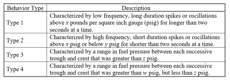Table 1 – A table containing the descriptions of the four problematic behaviors identified by AR engineering SMEs.

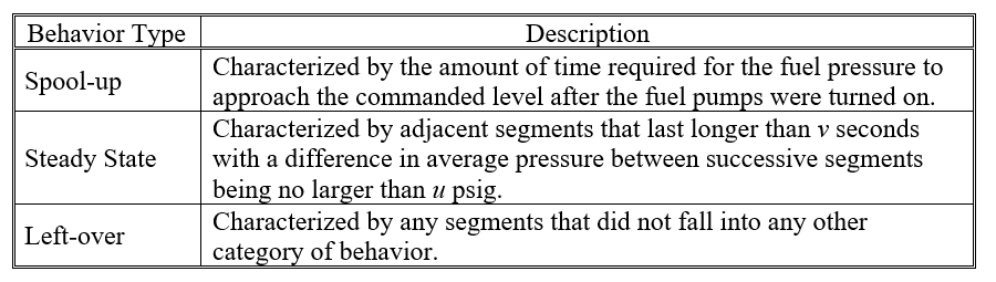Table 2 – A table containing the descriptions of the three non-problematic behaviors identified by AR engineering SMEs.

We note that it was possible to have a length of fuel pressure time series data be classified as multiple types of behavior simultaneously (e.g., Type 2 and Type 3 behavior are not mutually exclusive). Therefore, each of the above seven general types of behaviors required their own rules to recognize when the behavior started and stopped. Polymorphisms for the behavior types across multiple tankers and receivers also necessitated multiple sets of logic to identify the same type of behavior and a deterministic inference engine to identify and deconflict duplicate or conflicting classifications. For example, not all forms of Type 2 behavior could be identified by a single set of characteristics or logic. A second set of logic was developed that was not dependent on differences in mean pressure between adjacent segments to identify the remaining cases of Type 2 behavior. The results of the two logic sets were deduplicated and combined. Figure 1 provides a visual of the order by which the inference engine passed pre-processed data segments through the logic sets, while deconflicting any contradictions. 

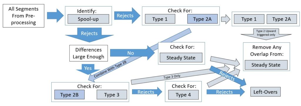
Figure 1: A diagram of the expert system flow and inference engine. Boxes represent logic sets that identify behavior types or categorize the data segments in some way. Arrows represent the movement of data through the expert system flow. Dark blue arrows are associated with moving data between logic sets that classify behaviors, while light blue and gray arrows move data through logic sets that eliminate redundancies and address contradictions in classification, respectively. Segments that were not classified as “spool-up” behavior are simultaneously fed through two separate branches of the ES and inference engine before contradictions are resolved.

After the ES has processed all the fuel pressure segments, the system output consists of a matrix of start and end times for each type of behavior and an identifier to map each instance of behavior back to the associated data segments. An analyst can then use a separate function to compile statistics about the prevalence of each type of behavior or groupings of similar behaviors (e.g., all behaviors that qualify as Type 1-4), and conduct other statistical analyses by behavior groups to support evaluation of the AR system.

The PELT algorithm and ES together form the Fuel-pressure Artificial intelligence Classification System (FACS). The FACS identifies various fuel pressure behaviors, including their beginning and end, as shown in Figure 2.

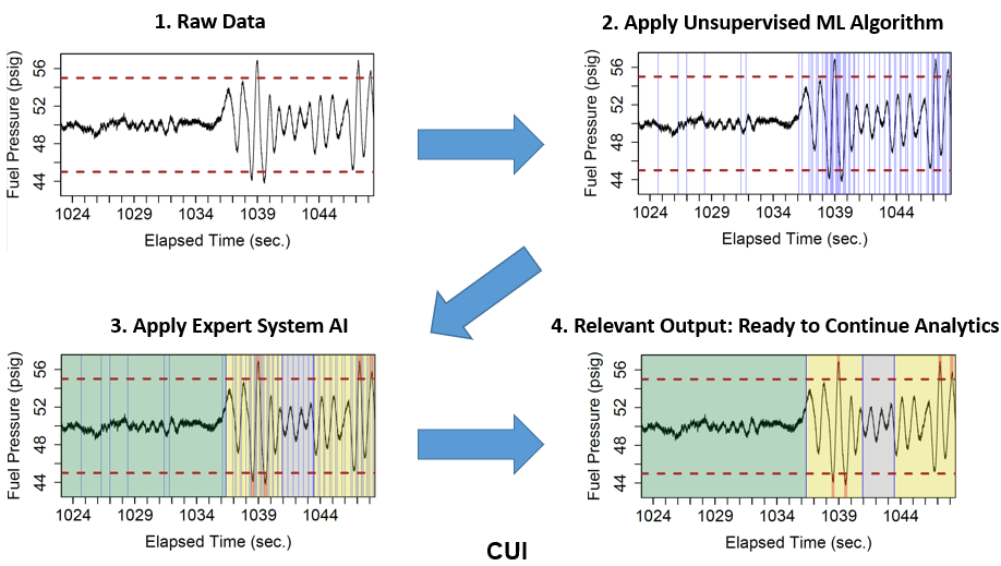
Figure 2: A simplification of how a fuel pressure data stream is analyzed by the FACS. 1) Raw data is provided to the FACS; 2) the PELT algorithm estimates the locations of changepoints; 3) the ES classifies fuel pressure segments as various behavior types; 4) the ES provides the start and stop times for each instance of any fuel pressure behavior that is present in the data stream. Segments highlighted in green are steady state. Yellow segments denote Type 1-4 behavior. Gray segments denote left-over behavior.

Grogono and Suen (1993), Frishkoff, et al. (2007), and Miranda et al. (2011) all propose methods for validating and evaluating the performance of aspects of an ES. Grogono and Suen (1993) advocates for functional testing and structural testing. In functional testing, each aspect of ES functionality is checked using test cases of varying difficulty levels. In structural testing, test cases are built to show that all aspects of the ES order of operations execute as designed and expected. At every step of development, we employed both functional and structural tests on the FACS ES. We solicited feedback from SMEs at every development iteration to improve performance. Perhaps unsurprisingly, the iterative feedback elicited numerous refinements to fuel pressure behavior definitions as well as requests for additional functionality.

Classifying fuel pressure behaviors in AR requires elements of objectivity and subjectivity. As a result, no gold standard of performance for the FACS exists, per se. Rather, the utility of the FACS in this situation is the reproducibility, defensibility, and consistency of applying the same logical rule sets across fuel pressure data regardless of when they were collected. In the absence of objective measures of validity, Grogono and Suen (1993) recommends employing an agreement method – that is, compare the quality of classifications from the FACS against that of one or more SMEs. We provide a side-by-side comparison of SME classification work against FACS work in the next section.

A final challenge in operational testing is picking the values for the tunable FACS hyperparameters, such as the shape for the gamma distribution in the PELT algorithm, and the difference in mean pressure between adjacent segments required to allow segments to be checked for Type 2-4 behavior. The gamma shape parameter influences what differences in fuel pressure from one observation to another are large enough to necessitate inserting a changepoint. The difference in mean pressure parameter acts similarly to a penalty and influences how large the difference in mean fuel pressures between adjacent segments must be to distinguish between steady state and certain transient behaviors (i.e., Type 2-4). We learned while developing the FACS that these hyper-parameters are correlated (the setting of one hyper-parameter affects the optimality of the value of another hyper-parameter) and must be adjusted depending on the type of tanker that passes fuel and/or the type of receiver being refueled. For example, we learned certain hyper-parameter values enabled quality fuel pressure classification for smaller, lighter fighter aircraft, while a slightly different set of hyper-parameter values worked better for larger, heavier cargo aircraft. We gained this knowledge via diligent functional test experience. Tracking the summary statistics about total time classified into each behavior type across different hyper-parameter values, combined with visual and SME checks, can provide a sense of which hyper-parameter values give stable performance.

We now compare fuel pressure classification output from FACS against the work of an AR engineer. The examples we provide are fuel pressure time series data collected during boom AR certification for three different tanker/receiver pairings: Tanker A paired with Receiver 1, Tanker A paired with Receiver 2, and Tanker B paired with Receiver 3. The data were collected by the Global Reach Combined Test Force at Edwards Air Force Base, California between 2010 and 2023. For simplicity, we focus on three behaviors that are of most concern: Type 1, Type 2 that crosses above 55 psig, and Type 3. We show plots of approximately forty seconds of labeled FACS output compared to AR engineer judgements for each pairing and discuss our observations.

First, we examine data collected from Tanker A paired with Receiver 1 in Figure 3. This period contains Type 1-3 behaviors. While both the AR engineer and FACS identify areas of Type 1-3 behavior, the FACS can simultaneously identify multiple types of behavior that are layered over each other to provide a more thorough analysis.

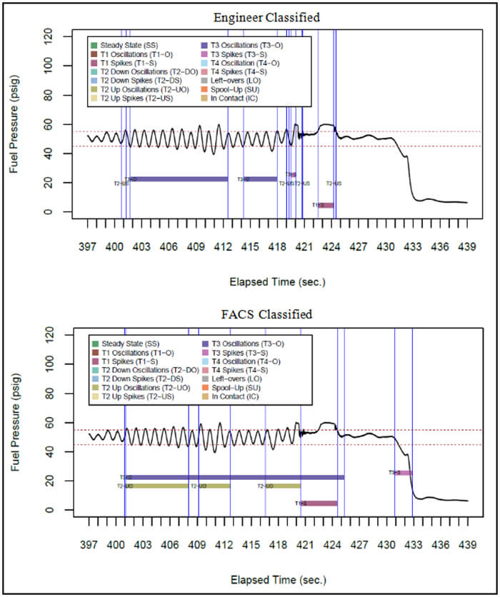
Figure 3: A comparison of how an AR engineer classified fuel pressure behavior for Tanker A and Receiver 1 versus the FACS.

Next, we examine data collected from Tanker A paired with Receiver 2 (TAR2) in Figure 4. This period contains complex Type 2-3 behaviors. Again, both the AR engineer and FACS identify areas of Type 3 behavior. Where the engineer identifies the behavior starting at 1582 seconds as a single stretch of Type 3 oscillation, the FACS breaks this period into two separate Type 3 oscillations and one Type 3 spike. Conversely, the engineer only identifies one area of Type 2 spiking, while the FACS identifies every instance that fuel pressure rose above 55 psig as a Type 2 spike.

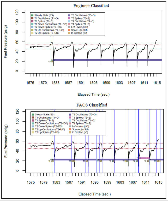
Figure 4: A comparison of how an AR engineer classified fuel pressure behavior for Tanker A and Receiver 2 versus the FACS.

Last, we examine data collected from Tanker B paired with Receiver 3 in Figure 5. This period contains Type 1-3 behaviors. While the AR engineer identified Type 3 behavior throughout the data stream, they did not identify the Type 2 behavior at 496 seconds and misidentified Type 1 behavior as starting around 517 seconds instead of 502 seconds. The FACS subdivided the period from 495-502 seconds into several types of behavior based on the tiny oscillations found around 498 seconds that ended the Type 2-3 behaviors. 

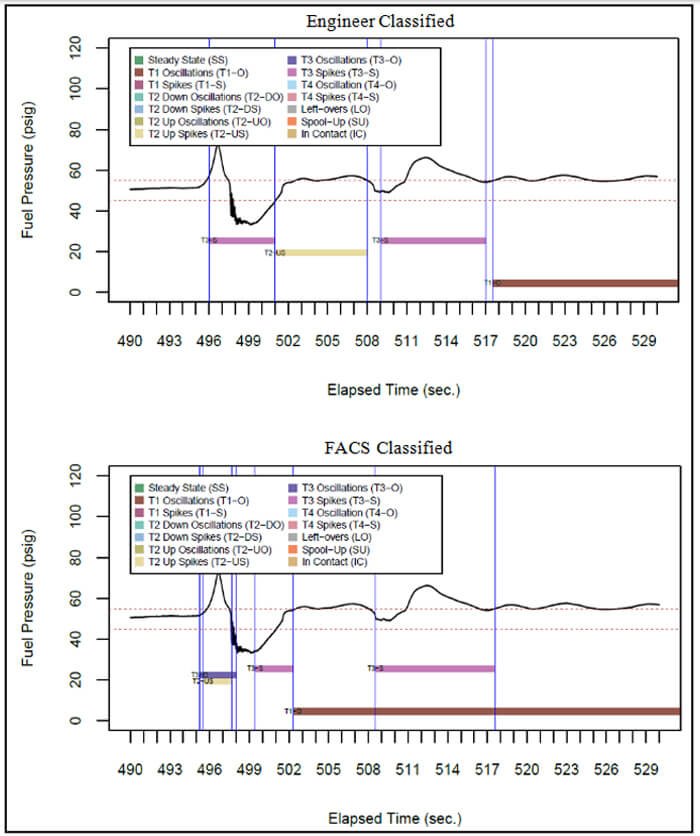
Figure 5: A comparison of how an AR engineer classified fuel pressure behavior for Tanker B and Receiver 3 versus the FACS.

In general, we glean several thoughts from the comparison of the FACS vs. AR engineer classification work. First, the engineer and FACS provided comparable classification work in most cases. Second, an AR engineer seems more able to identify broad patterns without bogging down in the minutia of extremely local behaviors, as evidenced from the TAR2 example in Figure 4. Third, an AR engineer seems less likely to correctly estimate precise quantities that determine the difference between certain types of behavior, like Type 1 and Type 2 behavior (fuel pressure above x psig for longer than two seconds at a time vs. shorter than two seconds at a time, respectively). Fourth, an AR engineer has difficulty identifying more than one behavior type at once in the same segments of data. Lastly, the FACS has an implicit weakness of occasionally needing to be calibrated if it encounters unique polymorphisms of Type 1-4 behaviors that were unseen or unknown during development. In this event, the logic within the ES would need to be enhanced to successfully classify the previously unseen forms of Type 1-4 behaviors moving forward. Regression testing would also be necessary to ensure that these logical changes would not degrade legacy functionality. 

Once the initial calibration of the FACS was completed, AR SMEs had an opportunity to review results and provide their perspective on the utility of the outputs. The SMEs found several aspects of the FACS to be particularly helpful. First, the FACS can process large data sets in a consistent manner and remove the subjectivity of each AR engineer performing data analysis. Second, the FACS provides detailed visual and categorical outputs which allow the AR engineers flexibility in their evaluations and reporting. Third, the FACS is more precise than an AR engineer can be when visually analyzing the data. Last, the FACS requires significantly less time (seconds) to complete an analysis than the manual reviews and discussions currently taking place (hours), resulting in a substantially smaller workload while improving the defensibility of the evaluations.

In this paper we have briefly discussed current challenges in defensibly and consistently classifying fuel pressure behaviors observed during AR certification operations. We have explained the difficulty of addressing this problem with widely used classification methods – namely that supervised classification requires authoritatively labeled fuel pressure data. We have explained how we addressed the behavior classification problem with the FACS, composed of a PELT changepoint detection algorithm and a tunable ES AI. We explained how AI like the FACS is typically validated when no authoritative truth source exists. Lastly, we showed that the FACS and an AR engineer make relatively similar judgements and discussed the difficulties, strengths, and weaknesses of the FACS approach. To date, the FACS provides a consistent, defensible, and repeatable analysis of fuel pressure data that substantially reduces engineer workload while improving the quality of the AR system evaluation.

The FACS system was trained using input from AR SMEs, a large set of AR data, and programming skill from statisticians and data scientists. However, the training data for the FACS is only a subset of fuel pressure time series data to which the FACS could be applied. As such, the FACS may require future refinements over time as unobserved behaviors could cause classification difficulties. In the future, one could train a reinforcement learning model on the output of the FACS and allow AR engineers to dispute questionable FACS judgements to continue improving the model over time. It is conceivable that the original FACS system (composed of the PELT algorithm and ES) could be replaced at some future time by the resulting reinforcement learning model. A system, similar to the FACS, may be created to provide consistent, defensible, and repeatable analysis of other subsystems, such as hydraulic pressure, electrical voltage, or oil pressure.

We thank the Global Reach Combined Test Force of the 412 Test Wing at Edwards AFB for providing the data, the technical experts, and the time to explore this problem. We thank Kevin Bailey and Wendy Peterson for their feedback on early ideas for the FACS. We thank the AR engineering staff for their time and efforts in assisting with and providing feedback on this effort. We thank the statistical methods flight of the 412 Test Wing for their feedback and guidance. Lastly, we thank two anonymous reviewers for their feedback that improved the quality of the manuscript. Any mention of products or services are for explanation purposes only and do not constitute an endorsement by the United States Government. The opinions expressed in this article are solely the opinions of the authors and do not represent the policy or opinion of the United States Government.

Aminikhanghahi, S., & Cook, D. J. (2017). A survey of methods for time series change point detection. Knowledge Information Systems, 339-367.
Aronson, J. E. (2003). Expert Systems. In H. Bidgoli (Ed.), Encyclopedia of Information Systems (pp. 277-289). Elsevier.
Copeland, B. (2018). MYCIN: artificial intelligence program. Encyclopedia Britannica. Retrieved March 29, 2023, from https://www.britannica.com/technology/MYCIN
Frishkoff, G. A., Frank, R. M., Rong, J., Dou, J., Dien, J., & Halderman, L. K. (2007). A Framework to Support Automated Classification and Labeling of Brain Electromagnetic Patterns. Computational Intelligence and Neuroscience, 2007, 1-13. doi:10.1155/2007/14567
Grogono, P., & Suen, C. (1993). A review of expert systems evaluation techniques. Association for the Advancement of Artificial Intelligence.
Hayes-Roth, F., Waterman, D. A., & Lenat, D. B. (1983). Building Expert Systems. Massachusetts, USA: Addison-Wesley Publishing Company.
Killick, R., & Eckley, I. A. (2014). changepoint: An R Package for Changepoint Analysis. Journal of Statistical Software, 58(3), 1-19. doi:10.18637/jss.v058.i03
Killick, R., Fearnhead, P., & Eckley, I. A. (2012). Optimal Detection of Changepoints With a Linear Computational Cost. Journal of the American Statistical Association, 107(500), 1590-1598. doi:10.1080/01621459.2012.737745
Leonard-Barton, D., & Sviokla, J. (1988, March). Putting expert systems to work. Harvard Business Review. Retrieved from Putting Expert Systems to Work.
Miranda, P., Isaias, P., & Crisostomo, M. (2011). Evaluation of expert systems: the application of a reference model to the usability parameter. In C. Stephanidis, Universal Access in Human-Computer Interaction, Part 1, HCII 2011, LNCS 6765 (pp. 100-109). Germany: Springer. doi:https://doi.org/10.1007/978-3-642-21672-5_12
Robinson, B. D., & Morrison, B. (2022). Online change-point detection for finding an anomaly in a high dimensional time series. United States Air Force, Air Force Research Laboratory, Sensors Directorate. Wright-Patterson Air Force Base: Air Force Research Laboratory. Retrieved Mar 1, 2023
Shortliffe, E. H. (1977). Mycin: A knowledge-based computer program applied to infectious diseases. Proceedings of the Annual Symposium on Computer Applications in Medical Care, (pp. 66-69).
Tartakovsky, A. G. (2014). Rapid Detection of Attacks in Computer Networks by Quickest Changepoint Detection Methods. In A. G. Tartakovsky, N. Adams, & N. Heard (Eds.), Data Analysis for Network Cyber-Security (pp. 33-70). London, UK: Imperial College Press.
Tartakovsky, A., Nikiforov, I. V., & Basseville, M. (2015). Sequential Analysis: Hypothesis Testing and Changepoint Detection. Boca Raton, Florida: CRC Press.
Wightman, J. (2022). Analytic case study using unsupervised event detection in multivariate time series. Air Force Institute of Technology, Department of Physics. Wright-Patterson Air Force Base: Air Force Intitute of Technology. Retrieved Mar 1, 2023
Wu, Z., Li, Lanye Hu, Y., & Hu, L. (2022). A synchronous multiple change-point detecting method for manufacturing process. Computers and Industrial Engineering, 108114. doi:https://doi.org/10.1016/j.cie.2022.108114