September 2023 I Volume 44, Issue 3
Experimental Design for Operational Utility
September 2023
Volume 44 I Issue 3
![]()
IN THIS JOURNAL:
- Issue at a Glance
- Chairman’s Message
Conversations with Experts
- Interview with Robert J. Arnold
Technical Articles
- I-TREE A Tool for Characterizing Research Using Taxonomies
- Scientific Measurement of Situation Awareness in Operational Testing
- Using ChangePoint Detection and AI to classify fuel pressure states in Aerial Refueling
- Post-hoc Uncertainty Quantification of Deep Learning Models Applied to Remote Sensing Image Scene Classification
- Development of Wald-Type and Score-Type Statistical Tests to Compare Live Test Data and Simulation Predictions
- Test and Evaluation of Systems with Embedded Machine Learning Components
- Experimental Design for Operational Utility
- Review of Surrogate Strategies and Regularization with Application to High-Speed Flows
- Estimating Sparsely and Irregularly Observed Multivariate Functional Data
- Statistical Methods Development Work for M and S Validation
News
- Association News
- Chapter News
- Corporate Member News

Abstract
Experimental Design for Operational Utility (EDOU) is a variant of Bayesian Experimental Design (BED) developed for principled cost/benefit analysis. Whereas traditional BED posits an information-based utility function, EDOU’s utility function quantifies the value of knowledge about a system in terms of this knowledge’s operational impact. Rough knowledge of important characteristics can matter more than precise knowledge of unimportant ones. EDOU assesses various testing options according to the tradeoff between the expected utility of the knowledge gained versus the cost of testing. When stakeholder priorities are captured in an operational utility function, it can recommend optimal decisions about which tests to conduct and whether further testing is worth the cost. The framework is illustrated with a simple example.
Keywords: Bayesian Experimental Design, Bayesian Decision Theory, Sequential Testing, Sequential Bayesian Analysis, Stochastic Dynamic Programming, Operational Utility
Introduction
An Experimental Design is a set of tests whose results are used to characterize system performance over a range of environments. These designs are typically formulated to either (a) estimate unknown system parameters or (b) predict future outcomes directly. Bayesian Experimental Design (BED) stipulates a prior probability distribution over system parameters, rather than treating them as simply “unknown.” This additional structure allows the knowledge gained from a test to be properly assimilated. The Bayesian versions of the estimation and prediction problems are computing (a) the posterior distribution over system parameters and (b) the posterior predictive distribution over outcomes.
Lindley formulated BED in terms of Bayesian Decision Theory (BDT) [1-3]. He treats experimental design as the optimization of some utility function. The estimation and prediction problems may both be handled in this BDT framework by specifying an appropriate utility function for each. In principle, Lindley’s approach could be used with a wide variety of utility functions, but in practice it tends to be used with either the information-based utility functions that arise in estimation and prediction, or else those derived from penalty functions used in optimization.
Experimental Design for Operational Utility (EDOU) follows Lindley’s approach but proposes a different philosophy for utility. EDOU is based on an acceptance utility function that quantifies how effective and suitable a system would be operationally given the current state of knowledge about its performance characteristics. This utility may be expressed in US dollars, or in any other lingua franca that allows all stakeholder priorities to be expressed. This use of common units enables principled cost/benefit analyses.
After the general framework for EDOU is presented below, it is illustrated via an example in which a simple hit/miss system is tested until the expected benefit of testing is outweighed by the cost of a test.
Framework
EDOU is presented in three parts. The first introduces the probability model. The second, the utility function; and the third, the decision procedure. The example in the next section will help clarify these ideas.
Probability model
Figure 1 shows EDOU’s Bayesian probability model. This model ingests outcomes y to update the knowledge κ about the system.
The figure uses plate notation to convey information about the various quantities [4]. It depicts a dataset comprising n pairs of context vectors x and outcomes y. The shading indicates that x and y are known data, while the rectangular “plate” indicates that there are n instances of (x,y). The square in Figure 1 indicates ξ has a fixed value; the circles indicate that all other quantities are random variables. The measurement likelihood function L(y|x,θ) specifies the probability density of the outcome y for a given context x [5].
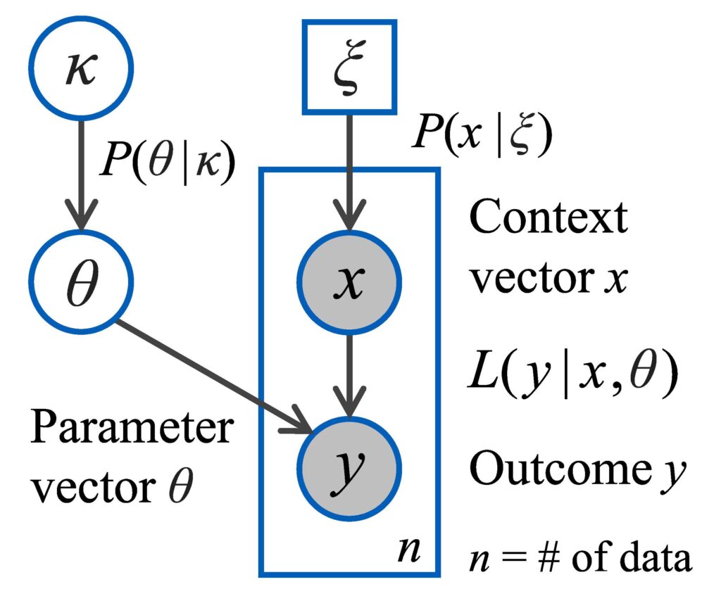
Figure 1 – EDOU’s Bayesian probability model.
Outcome y. An outcome y is the random result of a test. This can be as simple as the binary outcome y= “hit” or “miss.” Alternatively, y could be a non-negative real number representing an error (i.e., distance between target and impact) or a time until failure. The framework treats discrete, continuum, and more complex hybrid outcomes in a unified manner. For example, an outcome y may comprise a flag for “detected” or “undetected” plus additional data when detected. This data could include an error distance and a classification call. Whatever the form of the outcome y, the likelihood function L(y|x,θ) is formulated accordingly.1
Context vector x. The context vector x comprises all known conditions that may influence the random outcome y. It may include categorical information about the type of munition used or of the various settings for system configuration. The context may include the environmental conditions that are specified during test design, such as range, depth, and aspect angle. It may also include various conditions that can be measured during test but not planned, such as wind speed and temperature, though this is less useful for experimental design.
Parameter vector θ. The likelihood function L(y|x,θ) is specified by a parametric model, where θ comprises the model’s parameters. A common example is the linear Gaussian model which specifies that the scalar y has a Gaussian distribution with mean c∙x and variance σ2. The parameter vector is θ=(c,σ) in this case.
Knowledge κ. Classical statistics treats θ as an unknown quantity. Bayesian reasoning treats it as an uncertain quantity and specifies rules for uncertainty management. These rules are the unique extension of classical logic to handle uncertainty [6]. One’s current knowledge about θ is represented by κ via the probability distribution P(θ|κ). When the outcome y is observed for some context vector x, the knowledge κ is updated to some value κ+, producing an updated distribution P(θ|κ+). The distribution P(θ|κ) could have a specific functional form, such as the conjugate prior of L(y|x,θ). Another option is for κ to be a set of Markov Chain Monte Carlo (MCMC) samples of θ and for P(θ|κ) to be the reconstruction of the distribution (via Kernel Density Estimation, for example) [7,8].
Stakeholder priorities ξ. The final piece of the model shown in Figure 1 is the operational probability distribution P(x|ξ) over context vectors x. The parameter ξ represents stakeholder priorities. The distribution P(x|ξ) represents the importance that stakeholders attach to the system performing well in context x. A factor in this assessment is how often the context x would arise in practice, but stakeholders may also assign high importance to rarer contexts x due to the importance of the missions where these contexts occur.
EDOU’s probability model, shown in Figure 1, provides the mechanism for
- predicting how likely various outcomes y are in context x, given the knowledge κ, and
- updating the knowledge κ to some κ+ once an outcome y occurs.
The next part of the framework defines the value of having some state of knowledge κ. When combined with the probability model, this provides a mechanism for evaluating whether testing in some context x will tend to add value.
Utility function
Utility U. Let U(κ) denote the acceptance utility: i.e., the utility of accepting a system for which the distribution over the parameter vector θ is P(θ|κ). One may think of this as assessing the net benefit of putting the system into full-rate production and then deploying it, as is, with no further testing, relative to the alternative of rejecting it. More generally, U(κ) is the utility for acceptance into the next phase of testing given the current knowledge κ about the system.2 To make testing decisions, U(κ) must be expressed in the same units as testing costs.
The crux of EDOU is developing an appropriate acceptance utility U(κ) for a system being tested. The process of formulating U(κ) is a more detailed version of defining system requirements. It requires that stakeholders specify their priorities accurately to avoid situations where a system fails to meet the stated requirements but is accepted nevertheless because it provides sufficient value for the true mission of interest. Putting the EDOU framework into practice would require new elicitation methods for distilling stakeholder priorities into an acceptance utility U(κ). However, developing methods that clarify priorities would be effort well spent in improving the overall development and acquisition process. This subsection sketches three approaches to formulating U(κ), and the Example section below provides details for a simple case.
The first approach is based on using the posterior predictive probability density P(x,κ)=∫ L(x,θ)P(κ)dθ to formulate U(κ). One could assign a utility to each outcome y and then compute the expected utility using P(x,κ). This would provide a utility for κ in the context x, which one could then average over x using the operational distribution P(x|ξ). This is too simplistic, however. This procedure does not account for the fact that how, and whether, a system will be used depends on the knowledge κ one has about it. The Example section shows how this approach is modified to model how the knowledge κ is used. This is called the short-term utility formulation, denoted Us (κ).
The short-term utility is analogous to the prediction problem. In both cases the parameter vector θ plays no role: it is integrated out to form P(y|x,κ). The long-term utility formulation is analogous to the estimation problem. In this case, one considers the knowledge κ that emerges from testing to be only a short-term phenomenon. In the long-term, experience with the system will lead one to understand its performance characteristics well enough that (at least notionally) only the true value of θ will matter. In this case, the relevant short-term utility is the one based on L(y|x,θ), which may be denoted Us (θ). Although the true value of θ is unknown, P((θ)κ) provides its distribution, so the long-term utility is defined as UL (κ)=∫ Us(θ)P(θ)|κ)dθ.
A third approach to formulating U(κ) is as a compliance utility, denoted Uc(κ). This is a version of U(κ) that translates existing compliance requirements into a utility function. A compliance utility Uc(κ) takes one of only a few possible values. In the simplest case, it has a large value when κ satisfies the compliance criterion and a small value when it does not. When there are multiple criteria, Uc(κ) could be formulated as a sum of scores for each criterion met. Alternatively, if some criteria are mandatory, they would be left out of the sum, but Uc(κ) would be set to a small failure value if κ does not meet all mandatory criteria.
The acceptance utility function U(κ) encodes stakeholder priorities for accepting a system despite performance uncertainties. There are various approaches to formulating U(κ), three of which are listed above. Once the probability model in Figure 1 is specified, and U(κ) is developed, the final step is to leverage them to make optimal testing decisions.
Decision procedure
For a test event, one decides which tests to perform, executes them, updates one’s knowledge, and then decides whether to accept the system (into the next phase of testing) or to reject it. When decisions are made sequentially, this process is conducted repeatedly, with an additional “continue testing” option after each test (or suite of tests), until some final round n is reached and an accept/reject decision is required.
Action a. Let Ti be the set of possible testing actions a available after i rounds of testing are complete. The actions in Ti may be written a=A (Accept), a=R (Reject), or a=![]() . The first two are special cases in which testing stops immediately and the system is accepted or rejected. A proper testing action is an array of contexts x to test during round i+1, each of which will produce an outcome y. Such an action is written a=
. The first two are special cases in which testing stops immediately and the system is accepted or rejected. A proper testing action is an array of contexts x to test during round i+1, each of which will produce an outcome y. Such an action is written a=![]() , and the corresponding outcomes are
, and the corresponding outcomes are ![]() . Each action a∈Ti has an associated cost ca ≥ 0 which incorporates expended resources, usage of equipment, labor, etc. The special actions a=A and a=R have zero cost.
. Each action a∈Ti has an associated cost ca ≥ 0 which incorporates expended resources, usage of equipment, labor, etc. The special actions a=A and a=R have zero cost.
Let ui(κ,a) denote the expected utility of the system after round i of testing when the knowledge about the system is κ and the next testing action is to be a∈Ti. By definition,
ui(κ,A)=U(κ) and ui(κ,R)=0,
but the utilities for proper testing actions a=![]() are challenging to compute because they depend on the utilities from future rounds. The technique for solving for these utilities is Stochastic Dynamic Programming (SDP) [9]. Computing the utilities ui (κ,
are challenging to compute because they depend on the utilities from future rounds. The technique for solving for these utilities is Stochastic Dynamic Programming (SDP) [9]. Computing the utilities ui (κ,![]() ) using SDP entails two steps:
) using SDP entails two steps:
- Computing the update to κ given the outcomes
 , and
, and - Computing the corresponding utilities for these updated values of κ.
The first step is accomplished by updating the distribution P using Bayes’ rule:
P(θ|κ,![]() ,
,![]() ) ∝ L(
) ∝ L(![]() ,θ)P(θ|κ).
,θ)P(θ|κ).
There is often some conditional independence structure on ![]() that allows L(
that allows L(![]() |
|![]() ,θ) to be computed as a product of individual L(
,θ) to be computed as a product of individual L(![]() |
|![]() i,θ). This posterior distribution on θ is then converted into the chosen knowledge representation. In simple cases, P(θ|κ) can be chosen as a conjugate prior to the likelihood function L(y|x,θ) so the posterior P(θ|κ,
i,θ). This posterior distribution on θ is then converted into the chosen knowledge representation. In simple cases, P(θ|κ) can be chosen as a conjugate prior to the likelihood function L(y|x,θ) so the posterior P(θ|κ,![]() ,
,![]() ) will be of the same functional form as the prior. That is, it may be written exactly as P(θ|κ+) for some hyperparameter κ+ that can be computed directly. Otherwise, one can use MCMC or Variational Inference to compute an updated value κ+ such that P(θ|κ+) approximates P(θ|κ,
) will be of the same functional form as the prior. That is, it may be written exactly as P(θ|κ+) for some hyperparameter κ+ that can be computed directly. Otherwise, one can use MCMC or Variational Inference to compute an updated value κ+ such that P(θ|κ+) approximates P(θ|κ,![]() ,
,![]() ).
).
Let κ+(κ;![]() ,
,![]() ) denote the function that processes κ,
) denote the function that processes κ, ![]() , and
, and ![]() into the updated knowledge κ+. The distribution on the values of κ+ that arise from a given value of κ under the testing action a=
into the updated knowledge κ+. The distribution on the values of κ+ that arise from a given value of κ under the testing action a=![]() is now fully characterized because κ and
is now fully characterized because κ and ![]() are specified and the distribution on
are specified and the distribution on ![]() is
is
![]()
For the second step, some additional notation is required. Let ![]() (κ) denote an action a∈
(κ) denote an action a∈![]() that maximizes
that maximizes ![]() (κ,a), and let
(κ,a), and let ![]() (κ)=
(κ)=![]()
![]() (κ,a) =
(κ,a) = ![]() (κ,
(κ,![]() (κ)) denote this maximal utility. These are simple to compute for the terminal round n. In this case
(κ)) denote this maximal utility. These are simple to compute for the terminal round n. In this case ![]() ={A,R} because no testing is allowed after round n. Therefore
={A,R} because no testing is allowed after round n. Therefore ![]() (κ)=A when U(κ)>0 and
(κ)=A when U(κ)>0 and ![]() (κ)=R when U(κ)<0.3 Likewise,
(κ)=R when U(κ)<0.3 Likewise, ![]() (κ)=max(U(κ),0). In general,
(κ)=max(U(κ),0). In general, ![]() (κ)≥0 because the zero-utility option a=R is always available.
(κ)≥0 because the zero-utility option a=R is always available.
The value of ![]() (κ,a) may now be computed for 0 ≤ i < n in the case a=
(κ,a) may now be computed for 0 ≤ i < n in the case a=![]() :
:
![]()
Note that this recursion for the utility of the testing action a=![]() includes its cost c
includes its cost c![]() . If this cost is too large, then
. If this cost is too large, then ![]() (κ,
(κ,![]() ) will be negative for all context vectors
) will be negative for all context vectors ![]() , and testing will end.
, and testing will end.
The framework for EDOU has now been described. It consists of
- The probability model shown in Figure 1,
- The definition of the acceptance utility function U(κ),
- The update mechanism κ+(κ;
 ,) for the knowledge κ, and
 - The backward recursion for updating
 (κ,a) and computing the maximal utility
  (κ).
(κ).
EDOU provides optimal testing decisions. After any round i of testing, given the system knowledge κ, EDOU provides an optimal testing action ![]() (κ) to take. An optimal action a∈Ti is one that maximizes
(κ) to take. An optimal action a∈Ti is one that maximizes ![]() (κ,a). The utilities
(κ,a). The utilities ![]() (κ,a) themselves provide guidance for making on-the-fly modifications to a test plan: unforeseen circumstances may warrant making slightly sub-optimal choices, but not significantly sub-optimal ones.
(κ,a) themselves provide guidance for making on-the-fly modifications to a test plan: unforeseen circumstances may warrant making slightly sub-optimal choices, but not significantly sub-optimal ones.
Example
The EDOU framework is powerful and flexible, but rather abstract. This section provides an example of how the four steps of the EDOU process listed above may be applied to a simple scenario in which a system’s hits and misses are tallied. The goal is to determine when to stop testing the system and whether to accept or reject it.
The version of the probability model from Figure 1 tailored to this problem is shown in Figure 2. In this case the outcome y is a Bernoulli random variable taking the values “hit” or “miss.” The parameter vector θ has only the single entry p which represents the unknown hit probability. The measurement likelihood function is L(hit|p)=p and L(miss|p)=1-p. There is no context x to affect the outcomes. The beta distribution is the conjugate prior of the Bernoulli distribution, so this is the natural choice for P(θ|κ):
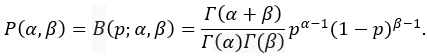
Thus the hyperparameter is κ=(α,β).
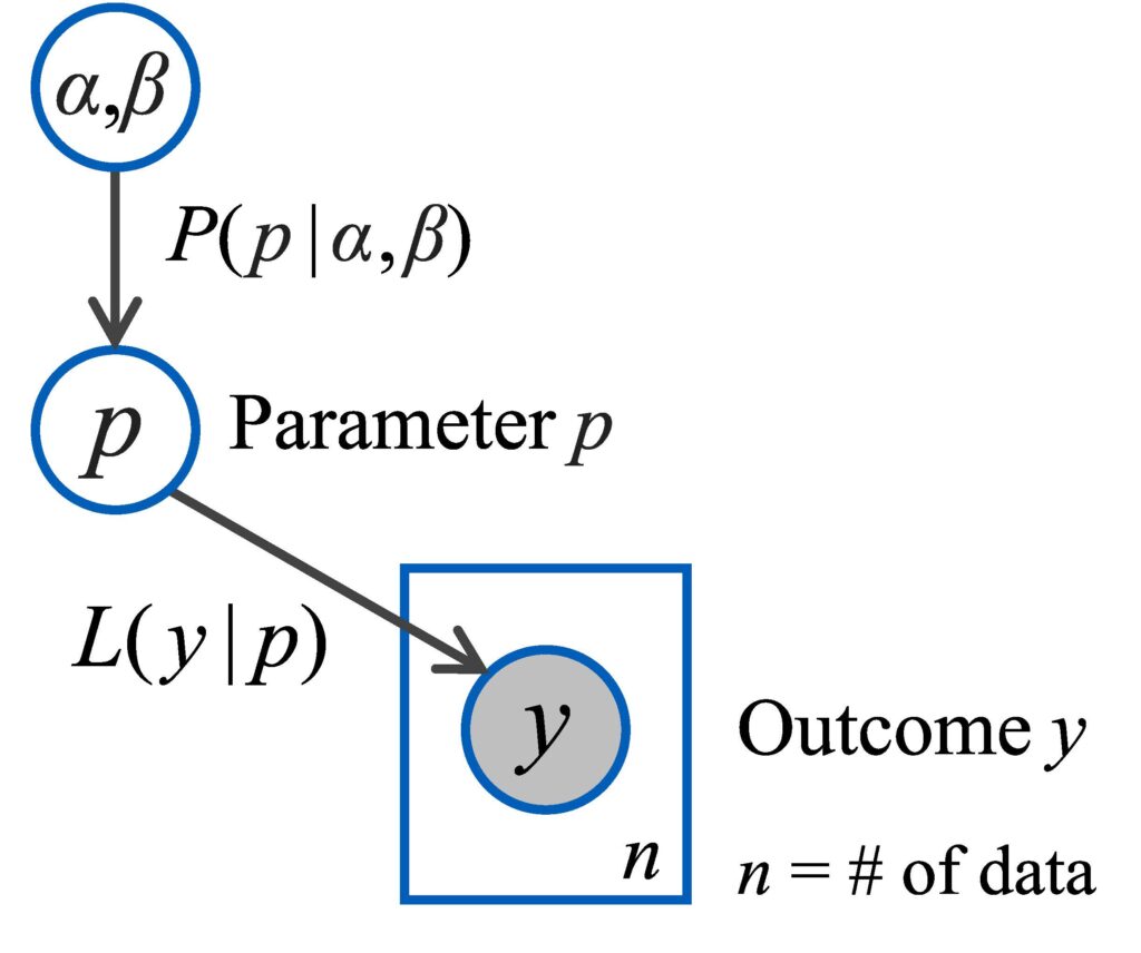
Figure 2: Probability model for example
The next step is to formulate the acceptance utility function U(κ)=U(α,β). This may be done using a short-term, long-term, or compliance utility. The posterior predictive distribution on the outcome y is a Bernoulli distribution with hit rate ![]() , so the short-term utility may be expressed as
, so the short-term utility may be expressed as ![]() . The model for
. The model for ![]() is
is

This model arises from a stylized scenario in which the system is available in a variety of situations with different payoffs for success. The value of p makes it worthwhile to use the system in some subset of these situations. The function ![]() increases with p from US(0)=-C0 to US(1)=U1, where C0=10 is the cost of producing the system, and U1=50 is the net utility of the system when p=1. The function decreases as s increases, and the value s=332.3 is chosen for the example illustrated below. The long-term utility function is
increases with p from US(0)=-C0 to US(1)=U1, where C0=10 is the cost of producing the system, and U1=50 is the net utility of the system when p=1. The function decreases as s increases, and the value s=332.3 is chosen for the example illustrated below. The long-term utility function is ![]() .
.
The compliance utility is defined to be Uc(α,β)=20 when at least Pcont of the probability mass of P(α,β) lies above p=pcut, where Pcont=0.95 and pcut=0.8. Otherwise Uc(α,β)=-10. The compliance utility makes a sharp jump between the values -10 and 20. The short- and long-term utilities instead vary smoothly and assign high utility to very accurate systems. In practice setting the parameters for EDOU utility functions is a more detailed version of the procedure by which compliance criteria are currently set. Compliance utility comes closest to a direct translation of compliance criteria into a utility function.
The next step of EDOU is the update mechanism κ+ (κ;![]() ,
,![]() ) for the hyperparameter κ=(α,β). Because the beta distribution is the conjugate prior of the Bernoulli distribution, each hit simply increases α by one and each miss increases β by one. Thus the update mechanism may be written κ+(α,β;hit)=(α+1,β) and κ+(α,β;miss)=(α,β+1).
) for the hyperparameter κ=(α,β). Because the beta distribution is the conjugate prior of the Bernoulli distribution, each hit simply increases α by one and each miss increases β by one. Thus the update mechanism may be written κ+(α,β;hit)=(α+1,β) and κ+(α,β;miss)=(α,β+1).
The final step is the recursion for updating ![]() (κ,a) for the various possible testing actions a in
(κ,a) for the various possible testing actions a in ![]() . In this case
. In this case ![]() ={A,R,C} for i=0 to n-1 and
={A,R,C} for i=0 to n-1 and ![]() ={A,R}.4 That is, after each test, one may choose to accept the system, reject it, or continue testing until n rounds of testing are complete. After this, one must accept or reject the system.
={A,R}.4 That is, after each test, one may choose to accept the system, reject it, or continue testing until n rounds of testing are complete. After this, one must accept or reject the system.
The utilities of the accept and reject actions are ![]() (α,β,A)=U(α,β) and
(α,β,A)=U(α,β) and ![]() (α,β,R)=0. The utility of the continue testing action is
(α,β,R)=0. The utility of the continue testing action is

Here CT is the cost of a single test. The expectation is over the posterior predictive distribution on y, which is that y=hit with probability ![]() and y=miss otherwise. Therefore
and y=miss otherwise. Therefore

The optimal utility for i=n is ![]() (α,β)=max(U(α,β),0), and the optimal action is
(α,β)=max(U(α,β),0), and the optimal action is ![]() (α,β)=A when U(α,β)>0 and
(α,β)=A when U(α,β)>0 and ![]() (α,β)=R when U(α,β)<0. For 0≤i<n, the optimal utility is
(α,β)=R when U(α,β)<0. For 0≤i<n, the optimal utility is
![]() (α,β)=max(U(α,β),0,
(α,β)=max(U(α,β),0,![]() (α,β,C)), and an optimal action
(α,β,C)), and an optimal action ![]() (α,β) is whichever a∈{A,R,C} yields
(α,β) is whichever a∈{A,R,C} yields ![]() (α,β,a)=
(α,β,a)=![]() (α,β).
(α,β).
Results
The backward recursion above is solved for the case of n=100 tests, with a prior distribution on p of P(p)=Β(p;α0,β0 ) where α0=10 and β0=2.5.5 After observing h hits and m misses the distribution on p is P(p|α,β)=Β(p;α,β) with α=α0+ h and β=β0+m.
Figure 3 shows the utility 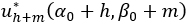 after h hits and m misses up to a maximum of h + m = 100 tests. The cost of each test is 0.01, so if all 100 tests are conducted, the total cost is 1: i.e., 2% of the maximum utility of the system itself. The utilities are computed using the long-term, short-term, and compliance utility functions. In each case the utility is zero whenever m≥27, so the long- and short-term plots are truncated.
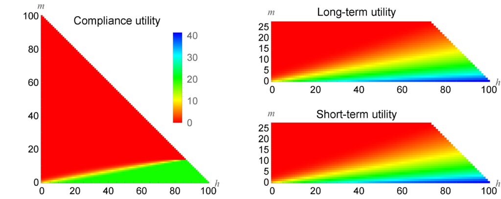
Figure 3: ![]() for three different acceptance utility functions with cT = 0.01
for three different acceptance utility functions with cT = 0.01
The optimal utility 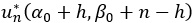 on the diagonals of these plots is zero for rejected systems and positive for accepted ones. In the compliance case, this positive utility is exactly 20. The values of 0 and 20 on the diagonal back-propagate through most of the utility plot, with an intermediate region in which this system is not yet accepted or rejected. The long- and short-term utility plots are much different from the compliance plot. In this case the utility of a system increases smoothly with its quality once that quality is above a certain threshold.
It is the local differences in utility that determine the optimal decisions, however. These differences are difficult to discern in Figure 3. Figure 4 plots the optimal decisions themselves. All possible pairs (h,m) of the numbers of hits and misses are color coded to form a decision chart. When there are h=5 hits and m=20 misses, all three charts color (h,m) red, indicating that the system should be rejected immediately.
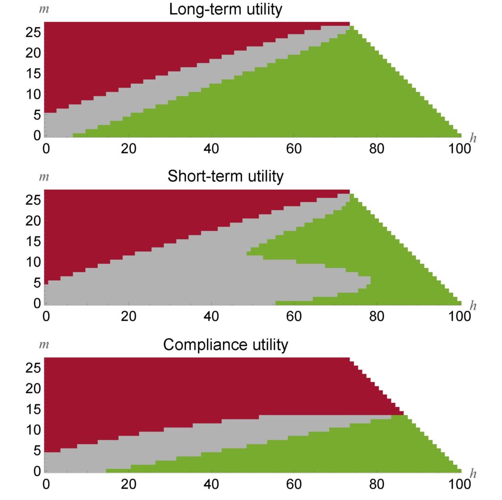
Figure 4 – Decision charts for cT = 0.01. Red = reject, gray = continue testing, green = accept
However, when there are h=70 hits and m=5 misses, the compliance and long-term charts color (h,m) green, indicating that the system should be accepted immediately, whereas the short-term chart colors it gray, indicating that testing should continue. All three charts have an upper gray lobe that prioritizes the need to distinguish between good and bad systems. However, the short-term acceptance utility function rewards a tight posterior distribution even for systems that will clearly be accepted. Because testing is inexpensive in this case, it recommends further testing in a lower gray lobe where testing has the largest impact on tightening the probability distribution over p.
Figure 5 shows the decision charts for a case where testing is 10 times more expensive. In this case, if all 100 tests are conducted, the total cost will be 20% of the value of an ideal system. In this case the gray “continue testing” regions tighten considerably for the long- and short-term utility functions, but only modestly for the compliance utility. This is because the all-or-nothing nature of the acceptance utility function in this case creates a strong incentive to continue testing even when it is expensive. This incentive also explains the long flat boundary between the red and gray regions in the compliance decision charts in Figure 4 and Figure 5. In these cases it is unlikely that testing will yield the dozens of consecutive hits without a miss that would be required to stay out of the red region, but the optimal decision is still to pay that testing cost for a small chance of a big payoff.
Figure 5 – Decision charts for cT = 0.1
Conclusion
Experimental Design for Operational Utility (EDOU) is a variant of Bayesian Experimental Design which employs a utility function that quantifies the value of knowledge about a system’s parameters in terms of the effect this knowledge will have in practice. In particular, the value of this knowledge is quantified in the same units as the cost of testing. Formulating the operational utility and testing cost in a common currency enables a principled cost/benefit analysis for testing.
The EDOU framework is illustrated with an example that compares three types of utility functions: long-term, short-term, and compliance. Although the example is quite simple, it demonstrates that the framework recommends fewer tests when testing is expensive. It also shows that different encodings of stakeholder preferences as utility functions leads to different optimal testing decisions. A utility function that places a premium on a tight parameter estimates even for clearly compliant systems will generate testing effort to tighten these estimates when the cost is sufficiently small and the information gain sufficiently large. Similarly, a utility function that imposes an artificially large distinction between barely compliant and barely non-compliant systems can generate test plans that spend too much effort to resolve this distinction.
Acknowledgement
This work was supported by The Director, Operational Test & Evaluation (DOT&E).
References
[1] Chernoff, Herman. 1972. Sequential Analysis and Optimal Design. Philadelphia, PA: Society for Industrial and Applied Mathematics.
[2] Chaloner, Kathryn, and Isabella Verdinelli. 1995. Bayesian experimental design: A review. Statistical Science 10 (3): 273–304.
[3] Atkinson, Anthony, Alexander Donev, and Randall Tobias. 2007. Optimum Experimental Designs, with SAS. Vol. 34. Oxford: OUP Oxford.
[4] Jordan, Michael I. 2004. Graphical models. Statistical Science 19 (1): 140–155.
[5] Gelman, Andrew, John B. Carlin, Hal S. Stern, David B. Dunson, Aki Vehtari, and Donald B. Rubin. 2013. Bayesian Data Analysis. 3rd ed. Boca Raton, FL: CRC Press.
[6] Jaynes, E. T. 2003. Probability Theory: The Logic of Science. Cambridge, UK: Cambridge University Press.
[7] Robert, C.P., and G. Casella. 2004. Monte Carlo Statistical Methods. 2nd ed. New York: Springer.
[8] Silverman, B. W. 1986. Density Estimation for Statistics and Data Analysis. London: Chapman and Hall.
[9] Bertsekas, Dimitri P. 2000. Dynamic Programming and Optimal Control. 2nd ed. Belmont, MA: Athena Scientific.
End Notes
1 L(y|x) denotes a probability density in general. When y is a discrete quantity, this simplifies to a probability.
2 It is simplest to think of U(κ) for the final phase of testing. To define U(κ) appropriately for earlier phases requires an analysis of subsequent phases. Thus, formulating U(κ) for multiple phases requires a macroscopic version of the backward recursion for utility that is performed within each phase.
3 Ties may be broken in an arbitrary manner: an* may be defined to be either A or R when U=0.
4 For consistency with general framework, C denotes the only possible proper testing action x: an array of length 1 containing the null context.
5 These parameters have been obtained, notionally, by imagining a previous round of testing that began with a uniform prior α=β=1 and then observing 12 hits and 2 misses to yield α=13 and β=3. However, a discount factor of 0.75 was applied because of changes in the system and testing environment to yield the values α=1+0.75×12=10 and β=1+0.75×2=2.5 that are used for the prior in the example.
Author Bio
Jim Ferry is a Senior Research Scientist at Metron, Inc. He has an SB in Mathematics from MIT and a PhD in Applied Mathematics from Brown University. He has been the Principal Investigator for a variety of projects for DARPA, ONR, and the intelligence community. His areas of expertise include Bayesian reasoning, network science, data fusion, and fluid dynamics.