More of the world is currently under high-resolution satellite and aerial surveillance than at any other time in history. Data of varying modalities is being recorded at an enormous rate; for example, data may come from multispectral or hyperspectral sensors, or sensors measuring visible wavelengths. The recent development of foundation models (FMs), e.g., transformer models, provides a potential avenue for addressing some data deluge challenges [1].

FMs are first trained on large diverse datasets, then, fine-tuned to a wide range of downstream tasks using smaller task-specific datasets. FMs were initially developed within the context of natural language processing (NLP) tasks and achieved remarkable performance on a wide range of NLP tasks, including language translation, text classification, and question answering. Recently, FMs have been broadened to computer vision tasks, such as object detection and segmentation. For example, Vision Transformer is a FM used for computer vision tasks [2]. Similar to FMs used for NLP tasks, FMs for computer vision tasks are pre-trained on large datasets, e.g., ground-based ImageNet imagery [3], and fine-tuned on task-specific data, e.g., satellite imagery [4].

The field of FMs is rapidly evolving. FMs have been extended to multi-modal data, such as a combination of text with images, video, or audio [5]. However, FMs also face some challenges. A prodigious computational requirement is one of them. FMs, in particular language FMs, tend to have many more parameters than CNNs. For example, the GPT-3 model developed by OpenAI has 175 billion parameters [6], and Switch Transformer developed by Google has 1.6 trillion parameters [7]. This limits their scalability and makes it difficult to deploy such models on resource-constrained devices.

A second challenge is evaluation of predictions beyond simple accuracy scores. Currently, many accuracy-based metrics, such as classification accuracy and F1-score, are used to quantify performance of FMs in applications. However, while accuracy-based metrics are important, predictive UQ and assessments of a model’s calibration are equally important. UQ and model calibration are related, but not identical. UQ refers to the process of estimating the level of uncertainty in a model’s predictions. This can include both data uncertainty and model uncertainty, with the latter arising from the model’s lack of knowledge or understanding of the true data generating mechanism. Model calibration, on the other hand, refers to the process of ensuring that a model’s predicted probabilities align with the true probabilities of the predicted events. A well-calibrated model will assign probabilities that reflect the true likelihood of the events occurring, and will typically have more accurate uncertainty estimates. In other words, a model that is poorly calibrated may overestimate or underestimate the uncertainty in its predictions, which can lead to incorrect decisions. Therefore, it is important to both evaluate a model’s calibration and quantify its uncertainty in order to ensure accurate and reliable predictions.

In this paper, we briefly review methods for test and evaluation (T&E) of FMs and perform a case study of T&E of ten deep learning models, including CNNs and transformer models, applied to the task of image scene classification using satellite and aerial imagery. We have chosen two transformer models because the transformer architecture is commonly used in FMs. It allows FMs to capture long-distance contextual dependencies in the data in a computationally efficient manner. Accounting for context in images is important because many activities of interest reveal themselves in co-occurrence of related image objects or related signatures spread over an extended areas (Fig. 1).

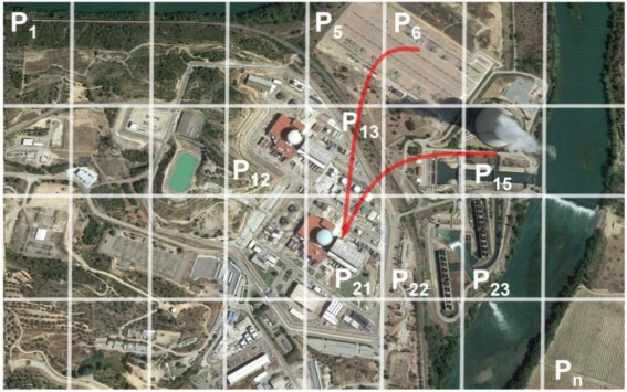
Figure 1. Illustration of capturing long-range dependencies. The image is partitioned into a set of pixel patches P₁ – P_n, and all inter-patch dependencies, e.g., outlined with red lines, are captured by a transformer model. The highlighted co-occurrence of a reactor building (in P₂₁), a cooling tower (in P₁₅), and an electrical substation (in P₅ and P₆) is used by a transformer to recognize a nuclear power plant. This is the image of Asco nuclear power plant, Spain, acquired July 2018. Image credit © Google Earth.

Transformer models serve as proxy models for larger-scale FMs of high complexity in terms of the number of model’s parameters. We target post-hoc evaluation of FMs, i.e., the evaluation of trained “black-box” models, when an end user does not have access to the internals of the model, but needs to know if the model is well-calibrated. For a more rigorous evaluation, we leverage image data augmentation methods. In Section 2, we review UQ approaches and metrics used for T&E of FMs, their constraints, and open problems. Section 3 summarizes computer vision tasks that are of interest for processing overhead imagery. Section 4 presents results of our case study. Finally, conclusions and directions for future work are presented in Section 5.

In this section, we discuss UQ methods and calibration methods that could be applicable to FMs. The goals of these techniques vary, from providing scalar measures of predictive variance, to providing prediction intervals (ranges of values that are likely to contain the true value), to providing full distributional predictions. In the context of FMs, some of these methods are unlikely to scale well, but each UQ method could also be applied only to a smaller submodel (e.g., the final hidden layer only) to achieve approximate results with reduced computational complexity. Commonly used UQ approaches include:

• Ensemble methods: Ensemble methods [e.g., 8] involve training multiple models with different initializations and/or architectures and combining their predictions, e.g., by taking the average or maximum prediction across all models. Variance in predictions across the ensemble can be used as a measure of model uncertainty. The choice of models to ensemble, the number of models in the ensemble, and the method of combining predictions impacts the performance and confidence of the ensemble model and required computational resources.
• Bayesian Deep Learning (BDL): BDL, including Bayesian neural networks, is a probabilistic approach that incorporates uncertainty into deep learning models [9, 10]. This approach involves placing a prior distribution over the parameters of the neural network, such as internode connection weights and node biases, which can be updated to a posterior distribution via approximate Bayesian inference, providing a full posterior distribution over model outputs that can be used to quantify the uncertainty in the model’s predictions. BDL encompasses a variety of methods for inferring posterior distribution, including variational inference [11, 12], drop-out variational inference [13, 14], sampling approaches [15-17], approximate inference based on Stochastic Weight Averaging Gaussian [18, 19], and Laplace approximations [20, 21]. Among drop-out techniques, Monte Carlo dropout [13] is often used.  Instead of only dropping out neural network units during training, dropout is also applied at test time, and multiple predictions are made for a given input, which can be used to calculate the variance in predictions. Bayesian methods can also be combined with ensembles, e.g., Bayesian nonparametric ensemble [22]. The computational complexity of BDL depends on the specific inference technique used, architecture and size of the model and the amount of data being used.
• Data augmentation (DA): DA involves applying different transformations to the input data during inference and averaging the predictions across the different transformations [23]. We can use DA both at training and test times. The latter is known as test-time data augmentation [24, 25], and can be used for post-hoc model evaluation and improvement. DA helps to estimate the uncertainty in the model’s predictions by measuring the variability across the different predictions. By making predictions on augmented versions of the input data and then computing the variance of the predictions, it is possible to estimate prediction intervals associated with the model’s predictions. It is important to note that the choice of data augmentation techniques can have an impact on the estimated prediction intervals. In Section 4, we show the use of data augmentation at test time as a practical method for testing and evaluating the predictions of deep learning models. 
• Sensitivity analysis (SA): SA is related to DA methods and involves adding noise or perturbations to the input data and measuring the impact on the model’s predictions and calibration [26-29]. SA can be used to identify which features have the most impact on the model’s prediction [30]. By permuting the values of each feature and measuring the change in the prediction, the importance of each feature can be estimated. 
• Bootstrapping: Bootstrapping is a resampling technique that can be used to estimate model uncertainty or assess the stability of a statistical estimate by creating multiple datasets through random sampling with replacement from the original dataset [31]. Bootstrapping can be used for both the train and test datasets, depending on the specific application and the question being investigated. Bootstrapping also provides variance measures and prediction intervals [32, 33].

Calibration encompasses post-hoc techniques to determine how well-calibrated a model is (i.e., how well the predicted probabilities reflect the true probabilities of the events being predicted), and to make corrections for miscalibrated models. Expected calibration error (ECE) [34, 35] and Brier score [38, 39] are metrics for evaluating the calibration of machine learning models used to assess the accuracy of the predicted probabilities and to identify potential issues with the calibration of the model.

The ECE is a scalar metric that measures the difference between the predicted probabilities and the actual frequencies of the events being predicted:

(1)

where n_b is the number of predictions in bin b of the histogram B and N is the size of the dataset,

(2)

is the predicted class label for event i obtained from the highest probability score, y_i is true class label, and is the highest probability score. Model predictions are partitioned on the range [0, 1] into separate bins bi based on their associated confidence scores. Due to the partitioning of model’s predictions, ECE is sensitive to the choice of binning.

ECE is closely related to reliability diagrams that represent model calibration by plotting accuracy as a function of confidence (Fig. 2) [35, 36]. The lower ECE, the better the model is calibrated. When ECE is 0, acc(b)=conf(b) for all bins. This is equivalent to all points falling on the diagonal line in the reliability diagram. While there are several approaches that try to address the binning choice, such as adaptive calibration error [37] and kernel density estimation, the choice of binning remains an open problem. The other challenge is that all the metrics can be affected by class imbalance.

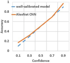
Figure 2. Illustration of reliability diagram for AlexNet CNN tested on the overhead imagery dataset RESISC45. A well calibrated model is represented by the diagonal line. Deviation from the diagonal indicates model’s miscalibration, such as under-confidence (points above the diagonal) or over-confidence (points below the diagonal) in model’s predictions.

The Brier Score (BS) measures the mean squared error between the predicted probabilities and the true labels. For multi-class predictions:

(3)

where K is the number of classes, Z_ik={0,1} is the indicator variable of class k for observation i, p_ik is the predicted probability of observation i to belong to class k. The lower the Brier score the better.

If a model is poorly calibrated, post-hoc techniques to correct the calibration can be applied. Confidence calibration techniques include temperature scaling, isotonic regression, ensemble calibration, and Bayesian calibration [e.g., 35, 40]. Confidence calibration is challenging. The open problems include: (1) calibration of the model under data shift, when the statistical properties of the training data and the test data differ, (2) time-varying calibration, when the underlying distribution of the data changes over time, (3) dealing with out-of-distribution samples, when samples do not belong to any of the known classes, (4) handling high-dimensional data, and (4) multi-class calibration.

We will present a case study in the image domain. In this section, we outline computer vision tasks of interest for remote sensing applications and order them based on the complexity of the analysis they require.

Image classification is an assignment of an entire image to a certain class or category, such as identifying whether an image contains a nuclear or coal-based power plant (Fig. 3). Localization goes a step further by not only identifying the object of interest but also drawing a bounding box around it to indicate its location in the image. Object detection is more complex as it requires localizing multiple instances of different objects in an image, often with overlapping bounding boxes. By detecting each individual object, we can count the number of instances of each object type, such as cooling towers and reactor buildings. Instance segmentation goes even further by not only identifying and localizing objects but also segmenting each instance of an object from its surroundings, by assigning a unique class ID and an instance ID to each pixel in the object of interest. Segmenting each individual instance of an object in an image allows for more accurate measurements of the object’s characteristics, such as its size, shape, and location relative to other objects in the scene. In contrast to the previous tasks, semantic and panoptic segmentations classify all the pixels in an image. Semantic segmentation labels each pixel of an image with a class ID, without differentiating between different instances of the same object class. Panoptic segmentation is the most complex, as it differentiates different instances and assigns an instance ID to each pixel.

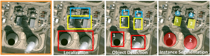
Figure 3. Illustration of image classification (e.g., whether the image contains a nuclear power plant or not), object localization, object detection and instance segmentation of different components of the nuclear power plant. Orange highlights that the image is classified as a whole. Red highlights cooling towers, yellow outlines turbines, and blue outlines reactors. Numbers represent IDs of individual instances of cooling towers, turbines, and reactor buildings.

These tasks build upon each other, with image classification providing a basic understanding of the content of an image, and instance and panoptic segmentations providing a detailed understanding of the spatial relationships between different objects in the image.

As a case study, we present results of the evaluation of the calibration of deep learning models, which provides a tangible example of the testing and evaluation of systems that rely on deep learning to automate tasks. We consider an application of CNNs and transformer models to remote sensing image classification, and compare the models using data augmentation, conventional metrics, such as classification accuracy, and calibration estimates using expected calibration error and Brier score.

For the evaluation, we use the publicly available and well-characterized Remote Sensing Image Scene Classification dataset (RESISC45) [4] (Fig. 4). We evaluate ten deep learning models that were either trained from scratch on the RESISC45, or were pre-trained on the ImageNet1K [3] image dataset (Fig. 5) followed by fine-tuning on the RESISC45 [41], during which the parameters of the final layers of the pre-trained models are updated while the parameters of the earlier layers are held fixed. RESISC45 dataset contains 31,500 images, covering 45 scene categories with 700 images in each category, and with spatial resolution that varies from 0.2 to 30 m per pixel. This dataset was collected over different locations and under different conditions and possesses rich variations in viewpoint, object appearance, spatial resolution, and background. The test dataset is a subset of RESISC45 and consists of 6,300 images with 140 images per category. Included in the categories are thermal power stations, storage tanks, parking lots, harbors, industrial areas, commercial areas, bridges, and airplanes. ImageNet1K is a benchmark in object detection and classification that spans 1,000 object classes and contains ~1.2 million images. The evaluated deep learning models include CNNs and transformers. Among the CNN models are earlier and broadly used models, such as AlexNet [42], VGG16 [43], ResNet50 and ResNet152 [44], DenseNet161 [45], and more recent models, such as EfficientNet [46], MLPMixer [47], and ConvNeXt [48]. FM-like transformer models are represented by Vision Transformer (ViT) [2] and Swin transformer [49].

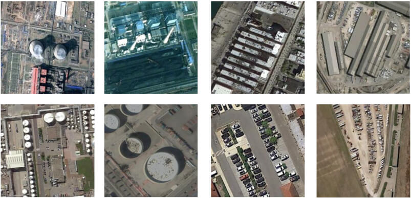
Figure 4. Image examples from RESISC45 dataset.

Figure 5. Image examples from ImageNet1K dataset.

We extend the evaluation of models by using augmented test datasets. We generate ten augmented test datasets, which are transformed copies of the original test dataset. Usually, data augmentation is performed when a model is being trained. Here, we perform augmentation in order to obtain more accurate estimates of model’s performance under perturbations to the image characteristics in the test data set. In particular, we use a combination of the following augmentations:

• Brightness: change a brightness by a magnitude drawn randomly from a uniform distribution over [-0.1, 0.4];
• Contrast: change a contrast by a magnitude drawn randomly from a uniform distribution over      [-0.1, 0.1]; and
• Rotation: rotate an image by an angle selected randomly from a uniform distribution over                 [-90, 90].

We limit the magnitudes of the contrast and rotation changes so that the transformed images remain close to the distribution of images in the original dataset. However, we intentionally allowed brightness to change more than is present in the original dataset to examine the impact of solar illumination and sensor viewing angle on model performance across a broader range of image acquisition conditions that could be encountered in practice.

Our results are summarized in Figs. 6 – 9. First, the results indicate that pre-training on a general large-scale dataset (shown by purple and red columns) does improve classification performance and calibration of all the evaluated models (Figs. 6-8). This is a consequence of including a more varied set of image acquisition conditions in a general dataset, especially in terms of brightness variation. Additionally, the variation (as indicated by length of error bars) in performance on augmented datasets is generally much larger for trained-from-scratch models, providing evidence of the robustness of a pre-trained model compared to a trained-from- scratch model. This also exemplifies the utility of data augmentation at test time as a method for investigating the robustness of systems that use deep learning models to automate tasks.

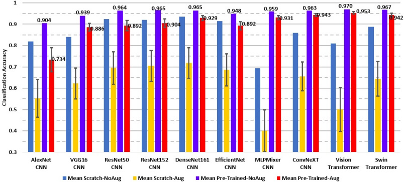
Figure 6. Classification accuracy of the models on the original and augmented test datasets. Blue column represents performance of the trained-from-scratch-on-task-specific-dataset models that were evaluated on the original non-augmented test dataset. Yellow column shows average performance and error bars (computed as standard deviation) of the same model across all augmented test datasets.  Purple and red columns represent performance of the pre-trained-and-fine-tuned models that were evaluated on the original test dataset and over all augmented test datasets, respectively. No error bars for blue and purple columns are given as the models were evaluated on only the original non-augmented test dataset.

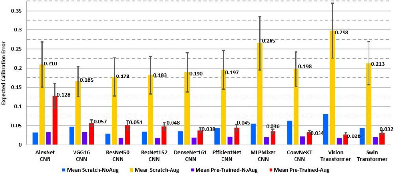
Figure 7. Expected calibration errors for the evaluated models. Column color coding is the same as in Figure 6.

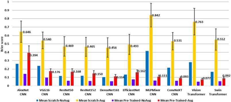
Figure 8. Brier scores, smaller is better, for the models trained from scratch and models pre-trained and fine-tuned. Column color coding is the same as in Figure 6.

Second, the transformers perform better than the CNN competitors when they are pre-trained and fine-tuned (Fig. 6). The transformers also exhibit smaller Brier scores and expected calibration errors, suggesting that they are better calibrated than other models (Figs. 7 and 8).

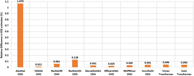
Figure 9. Relative difference in the Expected Calibration Error (ECE) estimates using 10 & 30 bins for the pre-trained & fine-tuned models on the original test dataset.

Third, the transformer models are more robust to changes in the image acquisition conditions that were simulated with data augmentation. This is particularly noticeable for the ResNet50 model. Pre-trained and fine-tuned ResNet50 models are close to the transformers in terms of accuracy, Brier score, and ECE when evaluated on the original non-augmented test dataset. However, when the evaluation is done on the augmented datasets, ResNet50 performs worse than the transformer models.

It is also interesting to note that, on the augmented test datasets, ConvNeXt, a CNN-like model recently designed to challenge transformer models, has shown performance comparable to the transformers and better performance than other CNN models (e.g., ResNet50). If evaluated only on the original test dataset without data augmentation, the ConvNeXT model would have a lower ranking than ResNet50. These results underscore the importance of data augmentation to obtain more precise evaluation.

Finally, Fig. 9 demonstrates the ECE dependence on the choice of binning. In our study, the difference in the ECE estimates using 10 and 30 bins is not significant both on the original and augmented datasets.

There are two main practical takeaways of this work that are relevant to the use of deep learning models for automating system tasks. The first is that pre-training a deep learning model on a large corpus of data followed by fine tuning on a task-specific data set yields better classification performance than training a deep learning model from scratch on the task-specific data set. The second is that data augmentation helps determine how robust a deep learning model is to perturbations in the test data, thereby better indicating how well a system based on a deep learning model will perform in practice than using a single, fixed test data set.

There are a number of ways to expand our study. Next steps include evaluating a model’s calibration on imbalanced datasets. This is important because training a model on an imbalanced dataset can introduce bias in the model’s predicted probabilities. It is also unlikely that we will have balanced datasets in real situations. Bootstrapping the test dataset combined with data augmentation is a potential approach to overcome class imbalance and to perform such evaluation. Going beyond post-hoc T&E includes examination of Monte-Carlo drop-out approaches, Bayesian deep learning, and ensemble methods.

UQ and deep model calibration are complex fields. The challenges stem from FMs’ complexity, data quality [e.g., 50], data distribution shift from training and test data, out-of-distribution samples, scalability of UQ methods, data fusion (e.g., combining electro-optical, synthetic aperture radar and hyperspectral image data), and a lack of real-world baselines for UQ and deep model calibration, among others. Recent reviews on UQ in deep learning [51, 52, 53] and work on developing baselines and metrics for evaluation of uncertainty estimates [54] and model’s robustness to distributional shift and out-of-distribution samples [55, 56] aim to address some of the identified challenges. Continued study in UQ of FMs is important for adopting of FMs in a wide range of applications.

The authors would like to acknowledge the US Department of Energy, National Nuclear Security Administration’s Office of Defense Nuclear Nonproliferation Research and Development (NA-22) for supporting this work.

1. Bommasani, R. et al. 2021. On the opportunities and risks of foundation models. arXiv preprint arXiv:2108.07258.
2. Dosovitskiy, A. et al. 2020. An image is worth 16×16 words: Transformers for image recognition at scale. arXiv preprint arXiv:2010.11929.
3. Russakovsky, O. et al. 2015. Imagenet large scale visual recognition challenge. International Journal of Computer Vision, 115, 211-252.
4. Cheng, G. et al. 2017. Remote sensing image scene classification: Benchmark and state of the art. Proceedings of the IEEE, 105(10), 1865-1883.
5. Akbari, H. et al. 2021. Vatt: Transformers for multimodal self-supervised learning from raw video, audio and text. Advances in Neural Information Processing Systems, 34, 24206-24221. 
6. Brown, T. et al. 2020. Language models are few-shot learners. Advances in Neural Information Processing Systems, 33, 1877-1901. 
7. Fedus, W. et al. 2022. Switch transformers: Scaling to trillion parameter models with simple and efficient sparsity. The Journal of Machine Learning Research, 23(1), 5232-5270. 
8. Lakshminarayanan, B. et al. 2017. Simple and scalable predictive uncertainty estimation using deep ensembles. Advances in Neural Information Processing Systems, 30.
9. Kendall, A., & Gal, Y. 2017. What uncertainties do we need in Bayesian deep learning for computer vision?. Advances in Neural Information Processing Systems, 30.
10. Clark, A. et al. 2015. Weight uncertainty in neural networks. In: Int. Conf. on Machine Learning.
11. Blei, D. M. et al. 2017. Variational inference: A review for statisticians. Journal of the American statistical Association, 112(518), 859-877.
12. Zhang, C. et al. 2018. Advances in variational inference. IEEE Transactions on Pattern Analysis and Machine Intelligence, 41(8), 2008-2026.
13. Gal, Y, and Ghahramani, Z. 2016. Dropout as a Bayesian approximation: Representing model uncertainty in deep learning. In Proceedings of the Int. Conference on Machine Learning, 1050-1059, PMLR.
14. Gal, Y., & Ghahramani, Z. 2015. Bayesian convolutional neural networks with Bernoulli approximate variational inference. arXiv preprint arXiv:1506.02158.
15. Chen, T., et al. 2014. Stochastic gradient Hamiltonian Monte Carlo. In Int. Conf. on Machine Learning, 1683-1691, PMLR.
16. Betancourt, M. 2019. The convergence of Markov chain Monte Carlo methods: from the Metropolis method to Hamiltonian Monte Carlo. Annalen der Physik, 531(3), 1700214.
17. Hernández, S. et al. 2020. Improving predictive uncertainty estimation using dropout-Hamiltonian Monte Carlo. Soft Computing, 24, 4307-4322.
18. Maddox, W. J. at el. 2019. A simple baseline for Bayesian uncertainty in deep learning. Advances in Neural Information Processing Systems, 32.
19. Seckler, H., & Metzler, R. 2022. Bayesian deep learning for error estimation in the analysis of anomalous diffusion. Nature Communications, 13(1), 6717.
20. Ritter, H. et al. 2018. A scalable Laplace approximation for neural networks. In 6th Int. Conf. on Learning Representations, ICLR 2018-Conference Track Proceedings (Vol. 6). 
21. Lee, J. et al. 2020. Estimating model uncertainty of neural networks in sparse information form. In Proceedings of the Int. Conference on Machine Learning, 5702-5713, PMLR.
22. Liu, J. et al. 2019. Accurate uncertainty estimation and decomposition in ensemble learning. Advances in Neural Information Processing Systems, 32.
23. Shorten, C., & Khoshgoftaar, T. M. 2019. A survey on image data augmentation for deep learning. Journal of Big Data, 6(1):1-48.
24. Kim, I., Kim, Y., & Kim, S. 2020. Learning loss for test-time augmentation. Advances in Neural Information Processing Systems, 33, 4163-4174.
25. Lu, H. et al. 2022. Improved Text Classification via Test-Time Augmentation. arXiv preprint arXiv:2206.13607.
26. Zhang, J., & Li, C. 2019. Adversarial examples: Opportunities and challenges. IEEE Transactions on Neural Networks and Learning Systems, 31(7):2578-2593.
27. Ahmed, U. et al. 2023. Robust adversarial uncertainty quantification for deep learning fine-tuning. The Journal of Supercomputing, 1-32.
28. Sobol, I. M. 1993. Sensitivity analysis for non-linear mathematical models. Math. Modeling Comput. Exp., 1, 407-414.
29. Sobol, I. M. 2001. Global sensitivity indices for nonlinear mathematical models and their Monte Carlo estimates. Mathematics and computers in simulation, 55(1-3), 271-280.
30. Covert, I. et al. 2020. Understanding global feature contributions with additive importance measures. Advances in Neural Information Processing Systems, 33, 17212-17223.
31. Efron, B. 2021. Resampling plans and the estimation of prediction error. Stats, 4(4):1091-1115.
32. Bahat, Y., & Shakhnarovich, G. 2020. Classification confidence estimation with test-time data-augmentation. arXiv e-prints, arXiv-2006.
33. Li, J. et al. 2022. Blip: Bootstrapping language-image pre-training for unified vision-language understanding and generation. In Proceedings of the Int. Conference on Machine Learning, 12888-12900, PMLR.
34. Naeini, M. P. et al. 2015. Obtaining well calibrated probabilities using Bayesian binning. In Proceedings of the AAAI conference on artificial intelligence, 29(1).
35. Guo, C. et al. 2017. On calibration of modern neural networks. In Proceedings of the Int. Conference on Machine Learning, 1321-1330, PMLR.
36. Niculescu-Mizil, A., & Caruana, R. 2005. Predicting good probabilities with supervised learning. In Proceedings of the Int. Conference on Machine learning, 625-632.
37. Nixon, J. et al. 2019. Measuring Calibration in Deep Learning. In CVPR workshops, 2(7).
38. Brier, G.W. 1950. Verification of forecasts expressed in terms of probability. Monthly weather review, 78(1):1-3.
39. Gneiting, T., & Raftery, A.E. 2007. Strictly proper scoring rules, prediction, and estimation. Journal of the American statistical Association, 102(477):359-378.
40. Ding, Z. et al. 2021. Local temperature scaling for probability calibration. In Proceedings of the IEEE/CVF Int. Conference on Computer Vision, 6889-6899.
41. Dimitrovski, I. et al. 2023. Current trends in deep learning for Earth Observation: An open-source benchmark arena for image classification. ISPRS Journal of Photogrammetry and Remote Sensing, 197, 18-35.
42. Krizhevsky, A., et al. 2012. Imagenet classification with deep convolutional neural networks. Advances in Neural Information Processing Systems, 25, 1097–1105. 
43. Simonyan, K., & Zisserman, A. 2014. Very deep convolutional networks for large-scale image recognition. arXiv preprint arXiv:1409.1556. 
44. He, K. et al. 2016. Deep residual learning for image recognition. In Proceedings of the IEEE Conf. on Computer Vision and Pattern Recognition, 770-778.
45. Huang, G. et al. 2017. Densely connected convolutional networks. In Proceedings of the IEEE Conf. on Computer Vision and Pattern Recognition, 4700-4708. 
46. Tan, M., & Le, Q. 2019. Efficientnet: Rethinking model scaling for convolutional neural networks. In Int. Conf. on Machine Learning, 6105-6114, PMLR. 
47. Tolstikhin, I. O. et al. 2021. Mlp-mixer: An all-mlp architecture for vision. Advances in Neural Information Processing Systems, 34, 24261-24272.
48. Liu, Z. et al. 2022. A convnet for the 2020s. In Proceedings of the IEEE/CVF Conf. on Computer Vision and Pattern Recognition, 11976-11986.
49. Liu, Z. et al. 2022. Swin transformer v2: Scaling up capacity and resolution. In Proceedings of the IEEE/CVF Conf. on Computer Vision and Pattern Recognition, 12009-12019.
50. Schmarje, L. et al. 2022. Is one annotation enough? A data-centric image classification benchmark for noisy and ambiguous label estimation. arXiv preprint arXiv:2207.06214.
51. Abdar, M., et al. 2021. A review of uncertainty quantification in deep learning: Techniques, applications and challenges. Information fusion, 76, 243-297.
52. Gawlikowski, J., et al. 2021. A survey of uncertainty in deep neural networks. arXiv preprint arXiv:2107.03342
53. Psaros, A.F., et al. 2023. Uncertainty quantification in scientific machine learning: Methods, metrics, and comparisons. Journal of Computational Physics, 477, p.111902.
54. Nado, Z. et al. 2021. Uncertainty Baselines: Benchmarks for uncertainty & robustness in deep learning. arXiv preprint arXiv:2106.04015.
55. Malinin, A. et al. 2021. Shifts: A dataset of real distributional shift across multiple large-scale tasks. arXiv preprint arXiv:2107.07455.
56. Tran, D. et al. 2022. Plex: Towards reliability using pretrained large model extensions. arXiv preprint arXiv:2207.07411.