September 2023 I Volume 44, Issue 3
Statistical Methods Development Work for M and S Validation
September 2023
Volume 44 I Issue 3
![]()
IN THIS JOURNAL:
- Issue at a Glance
- Chairman’s Message
Conversations with Experts
- Interview with Robert J. Arnold
Technical Articles
- I-TREE A Tool for Characterizing Research Using Taxonomies
- Scientific Measurement of Situation Awareness in Operational Testing
- Using ChangePoint Detection and AI to classify fuel pressure states in Aerial Refueling
- Post-hoc Uncertainty Quantification of Deep Learning Models Applied to Remote Sensing Image Scene Classification
- Development of Wald-Type and Score-Type Statistical Tests to Compare Live Test Data and Simulation Predictions
- Test and Evaluation of Systems with Embedded Machine Learning Components
- Experimental Design for Operational Utility
- Review of Surrogate Strategies and Regularization with Application to High-Speed Flows
- Estimating Sparsely and Irregularly Observed Multivariate Functional Data
- Statistical Methods Development Work for M and S Validation
News
- Association News
- Chapter News
- Corporate Member News
Statistical Methods Development Work for M&S Validation

Curtis Miller, PhD
Operational Evaluation Division at the Institute for Defense Analyses
![]()
![]()
Abstract
Modeling and simulation (M&S) environments feature frequently in test and evaluation (T&E) of Department of Defense (DoD) systems. Many M&S environments do not suffer many of the resourcing limitations associated with live test. We thus recommend testers apply higher resolution output generation and analysis techniques compared to those used for collecting live test data. Space-filling designs (SFDs) are experimental designs intended to fill the operational space for which M&S predictions are expected. These designs can be coupled with statistical metamodeling techniques that estimate a model that flexibly interpolates or predicts M&S outputs and their distributions at both observed settings and unobserved regions of the operational space. Analysts can study metamodel properties to decide if a M&S environment adequately represents the original systems. This paper summarizes a presentation given at the DATAWorks 2023 workshop.
Keywords:Modeling and Simulation; Space-filling designs; statistical modeling; data generation
Introduction
In this paper we describe recent recommendations by the Institute for Defense Analyses (IDA) regarding the use of data generated via modeling and simulation (M&S) to generate a statistical model characterizing the M&S tool’s predictions throughout the factor space, by collecting outputs with a space-filling experimental design that allows discovery of trends throughout the factor space (Wojton, et al. 2021, Haman and Miller 2023). Such a metamodel should be seen as a key product accompanying the M&S tool.
In operational testing (OT), M&S can supplement data obtained during live testing, but testers need to validate M&S predictions for M&S to be useful. Given that M&S often does not face the level of resourcing and output collection restrictions live testing must overcome (cost per run, need for test assets, event organization, scheduling, and similar issues), M&S observation collection approaches should be able to generate more outputs than testers would collect from live data. Space-filling designs (SFDs) enable the collection of outputs throughout the factor space, which can then be used for estimating statistical metamodels describing the M&S tool’s outputs. These metamodels can then be used for verification and validation (V&V) activities such as checking the plausibility of the M&S tool’s behavior, and planning live testing.
While this paper focuses on OT and V&V, metamodeling has many other uses, including in developmental testing or after testing has been concluded and equipment is being deployed. Metamodeling techniques are application agnostic and thus of general usefulness to the test and evaluation (T&E) community.
The Role of Modeling and Simulation in Operational Testing
The Director, Operational Test and Evaluation (DOT&E) in the United States Department of Defense (DoD) is responsible for overseeing operational testing (OT) of acquired systems by DoD. DOT&E reports on test adequacy and a system’s operational effectiveness, suitability, and survivability. According to United States Code Title X §4171, OT must include live data; M&S alone fails to qualify as adequate OT.
DOT&E risks making incorrect assessments of a system’s performance when they use M&S because M&S predictions may fail to align with reality. In order to accept M&S predictions as descriptive of operational performance, DOT&E needs a body of evidence describing the M&S tool. Testers call this process of collecting evidence “verification and validation” (V&V). To help control the risk associated with the use of M&S, DOT&E published guidance on what evidence it needs from V&V before it will agree to factor M&S predictions into its assessments and reports.
DOT&E wants operational testers to collect predictions and outputs from M&S tools to summarize their performance. DOT&E presented their expectations in two memos (Director, Operational Test and Evaluation 2016, 2017); their requirements for assessing an M&S tool include:
- Collecting data throughout the entire factor space using design of experiments (DOE) methodologies such as space-filling designs (SFDs) to help maximize opportunities for problem detection;
- Estimating metamodels1 with outputs generated according to an SFD to characterize M&S predictions throughout the factor space; and
- Quantifying the uncertainty associated with M&S predictions and interpolating M&S predictions between directly observed points.
DOT&E refrained from stating specifically what statistical methods should be used; too many situation-specific contingencies exist to make broad prescriptions in policy documents. Nevertheless, operational testers need guidance on what specific methods to use, and examples of what good statistical M&S analysis looks like. The Institute for Defense Analyses (IDA) has published papers suggesting statistical methods testers could use to meet DOT&E’s guidance (Wojton, et al. 2021, Haman and Miller 2023).While the IDA papers focus on the role of M&S metamodeling in the OT context, metamodels have other uses. Test planners can use metamodels to guide the selection of factors in a live test’s DOE. Metamodels can serve as subcomponents of other M&S tools—for example, a metamodel predicting torpedo performance could be used in a campaign-level model. They can also be used as a part of fleet operations and planning, for example to plan exercises, do wargaming, or even do tactical planning. Predicting the performance of important equipment in these contexts aids the effectiveness of these other activities, and a warfighter planning an engagement will take all the relevant information they can get. In many of these instances, some M&S tools are not available due to the time, expense, expertise, or even physical restrictions required to use the M&S itself. In such situations, the metamodel can be used to extend an M&S tool’s reach.
Modeling and Simulation Experimental Designs Should Cover the Operational Space
A design of experiment (DOE) is a plan for collecting observations for later analysis, including statistical analysis. The DOEs used for planning live testing optimize inference for a specific statistical model and try to minimize uncertainty in estimating the model’s key parameters. The statistical model optimized by optimal designs is usually a linear model, which may not permit much exploration of the relationship between factors and the response of interest beyond broad trends and general shapes.
Testers can collect outputs from M&S tools more easily than from live operational tests. Live testing challenges include
- unforeseen events producing deviations from the original test plans;
- unreliable equipment preventing testing;
- difficulty in knowing ground truth about the events of the test; and
- obtaining the test assets and personnel needed to conduct a live test.
Given the greater ease in collecting M&S outputs and the importance of validating M&S tools, testers should use different DOEs for M&S V&V than they would use for planning live tests. These DOEs should allow for discovery of local trends in the M&S operational space, not just overall trends.
Space-filling DOEs (SFDs) vary the design points more than DOEs used for live testing (such as factorial designs or D-optimal designs). Figure 3-1 displays the benefits of using an SFD. Rather than optimizing the conditions for estimating a specific statistical model, these designs spread design points throughout the entire operational space. This spread permits greater flexibility in statistical modeling; of particular relevance to this discussion, we can use statistical models that learn the shape of relationships between factors and response variables from the M&S outputs, rather than prescribing the relationships’ shapes, as must be done in DOEs for live testing.
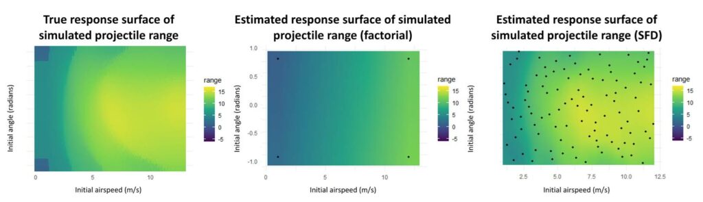 Figure 3-1: The plot in the left represents a true (unobserved in practice) response surface we want a statistical model to describe. A factorial design (middle plot) used with a linear model would fail to capture important characteristics of the surface, such as the multiple maxima of the surface or its ridges. The space-filling design (right plot), coupled with a Gaussian process statistical model, manages to recover these features.
Metrics describe how well a design fills space. One meaning of “space-filling” is that design points tend to be as far away from their neighbors as possible. The ‘maximin’ metric measures this point spread (Gramacy 2020) and thus describes this aspect of a design. Another meaning is that all regions of the operational space are equally represented by design points, with regions of equal volume having roughly the same number of design points. L2-discrepancy measures this uniformity of the design (Damblin, Couplet and Iooss 2013). Yet another meaning is that DOEs should be robust to dropping factors. The ‘MaxPro’ metric measures projection (i.e., sensitivity to dropping factors) (Roshan, Gul and Ba 2015). We have yet to see an SFD in statistical literature that replicates any design point or advocates for replication2, and replicating a factor does not yield as much utility to the resulting statistical model as spreading out points, so we prefer designs where the resulting design retains its space-filling properties even if a factor is ignored.
Most recommended designs are improvements on the basic Latin HyperCube Sampling (LHS) scheme. Many designs qualifying as LHS designs exist for a given set of factors and sample size, with many of those candidate LHS designs failing to match any intuitive notion of space-filling (for example, a design placing all points on a diagonal line counts as an LHS design). Test planners should pick an LHS that maximizes one of the space-filling metrics, such as the maximin-LHS (Damblin, Couplet and Iooss 2013).
While space-filling designs focus mostly on determining how to vary continuous factors, discrete factors (such as threat type, weapon type, day or night, and so on) need to be varied as well. Maximin-LHS designs generalize to the sliced maximin-LHS (maximin-SLHS) in order to accommodate categorical or discrete factors (Ba, Myers and Brenneman 2015). Maximin-SLHS designs would include a full factorial design to handle the categorical factors, which can result in impractically large sample sizes when test planners consider many categorical factors, and thus may restrict continuous factor variation; a MaxPro design based on an LHS design may better handle moderate to large numbers of categorical factors (Roshan, Gul and Ba 2015). A limitation of all of these designs is that they assume no restrictions on the factor space. Fast flexible filling (FFF) designs can easily account for such restrictions (Lekivetz and Jones 2019) while also providing a means for varying continuous factors. Figure 3-2 summarizes these space-filling design recommendations based on how well they optimize different evaluation metrics.
The ability to optimize a particular space-filling metric is not the only factor that must be considered when generating a design. Other important considerations include the number of continuous and discrete factors, and constraints on the operational space. Wojton et. al. (2021) and Haman and Miller (2023) summarize and recommend general purpose design generation methods based on the characteristics of the study.
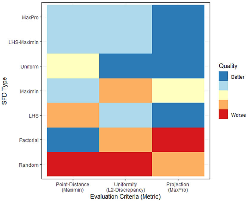
Figure 3-2: Space-filling design recommendation summary according to evaluation metrics. Wojton et. al. (2021) judged the quality of designs by studying metric properties and Monte Carlo simulation studies. Designs are evaluated based on how well they optimize some desirable metric describing the design: point-distance (the maximin metric), uniformity (described by L2-discrepancy), or projection (described by the MaxPro metric). Factorial designs include full factorial designs, potentially with much more than two levels for each continuous factor. Random designs sample points uniformly at random and independently from the factor space. Maximin designs spread points out such that the minimum distance between any two points in the design is maximized. Other designs are described in the paragraphs above.
Haman and Miller (2023) demonstrated SFD methodology with a hypothetical M&S study involving a paper airplane flight simulation.3 The study considers three factors:
- Initial airspeed of the paper airplane (continuous)
- The angle at which the airplane is thrown (continuous)
- The airplane design (categorical)
The paper airplane could be one of three models:
- The dart model
- The classic model
- A former world record paper airplane (WRPA) design.
Response variables include:
- Terminal range of flight (a continuous response)
- Whether a loop was observed in the flight path (a binary response)
Figure 3-3 displays the terminal range of flights through the factor space and shows that the response surface for this response variable features irregularities (ridges, multiple local maxima, curved surfaces) that a typical D-optimal design would fail to discover. In the hypothetical study, we will not be able to see the surface visualized in Figure 3-3, and will only be able to see responses at design points. Yet whatever statistical design is used should be able to recover the unique features of the response surface.
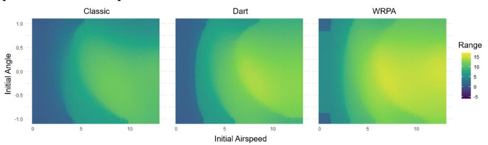
Figure 3-3: The relationship between terminal range of a paper airplane, depending on initial airspeed, initial angle, and the model of the paper airplane, as predicted by a numerical ordinary differential equation solver.
Figure 3-4 visualizes the 300-run maximin-SLHS used in Haman and Miller’s study (2023). Design points spread throughout the factor space, and the design uses no replicates. Such a design should discover local phenomenon that a typical D-optimal design would miss because the D-optimal design does not fill the space. The SFD better allows for discovery of interesting local phenomena in the M&S, provided that the outputs are analyzed with appropriate statistical models.
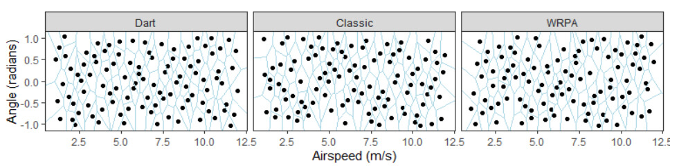
Figure 3-4: A maximin-SLHS SFD used in a hypothetical M&S study of a paper airplane simulation.
Flexible Statistical Models Describe Modeling and Simulation Behavior Generated by Space-filling Designs
After collecting M&S outputs, Haman and Miller (2023) recommend fitting a statistical metamodel to the observations. A metamodel summarizes M&S output with a statistical fit that interpolates or smooths the M&S output, essentially changing a complex computer simulation into a mathematical formula. While an M&S tool can require both physical infrastructure and millions of lines of computer code to support its operation, a metamodel might fit in the body of an email, almost certainly on the hard drive of a laptop. Statistical metamodels provide a framework for capturing uncertainty in typical M&S behavior, which matters when we need to compare M&S outputs to live test data. However, a metamodel only imitates the M&S output used in fitting; it may lack details of the physics involved in the situation that the M&S tool includes 4. Thus, the metamodel should be used in situations where its relative simplicity is essential to the activity.
Estimating a metamodel enables better OT and V&V. A statistical metamodel helps the consumers of M&S outputs understand the M&S tool’s overall behavior and identify where it may be producing problematic outputs. Metamodels alone are insufficient for validating an M&S tool; validation always requires live data. But a metamodel may give testers reason to believe that an M&S tool will not do well predicting real-world outcomes because the M&S outputs look implausible, alerting the M&S developers to the need to make adjustments before proceeding with further validation. In addition, a metamodel can help ensure the live data to be collected characterizes the equipment under study well. For example, the metamodel may suggest which statistical model should be used for planning live data collection. It may also recommend which regions live data collection should target. When live data are available, they may be compared against the metamodel to see if they agree with M&S predictions. DOT&E has recommended estimating statistical metamodels to characterize the M&S tool’s performance (Director, Operational Test and Evaluation 2017).
M&S tools have many characteristics and nuances, so analysts must identify appropriate statistical techniques when estimating a metamodel. The chosen statistical method should
- allow for interpolation between M&S observations in the factor space;
- characterize overall behavior;
- discover notable local phenomena in M&S behavior;
- provide for uncertainty quantification;
- robustly predict outputs other than the outputs used in statistical fitting; and
- produce information analysts can interpret.
Based on these requirements, Haman and Miller (2023) split their metamodeling recommendations based on the nature of the outputs generated by an M&S tool. They characterize M&S outputs as either discrete or continuous, and either deterministic or stochastic5. When outputs are deterministic, Haman and Miller recommend decision tree or nearest neighbor interpolators when the response variable is discrete (like the classification of a threat or whether a missile hits its target) (Hastie, Tibshirani and Friedman 2009); for continuous response variables (like miss distance), Haman and Miller recommend Gaussian process (GP) interpolation (Gramacy 2020). When outputs are stochastic, Haman and Miller recommend using generalized additive models (GAMs) for both discrete and continuous outputs (Wood 2017). These recommendations are summarized in Table 4-1. Note that the GAM framework includes the already commonly used linear models and generalized linear models (such as logistic regression), but extends the framework to allow for discovering the shape of trends in the typical response value from the data, rather than prescribing the shape like linear models usually do.
| Continuous Output | Discrete Output | |
| Deterministic Outputs | Gaussian Process (GP) | Nearest Neighbor or Decision Tree |
| Stochastic Outputs | Generalized Additive Model (GAM) | |
Table 4-1: Recommendations for statistical modeling approach based on M&S output type
GPs check most of the boxes for good metamodeling practice but lack the interpretability advantages of well-designed GAMs. For this reason, Haman and Miller (2023) recommended GPs only for the deterministic M&S situation where interpolation or near-interpolation is desired. Otherwise, a GAM is easier to fit and more interpretable.
Haman and Miller demonstrated these characteristics in their paper using the paper airplane simulation example. When they generated terminal range outputs from the deterministic version of the paper airplane simulation, they fit a GP to interpolate the outputs and obtained uncertainty estimates in the value of the interpolant at unobserved factor settings; we visualize the interpolation in Figure 4-1.
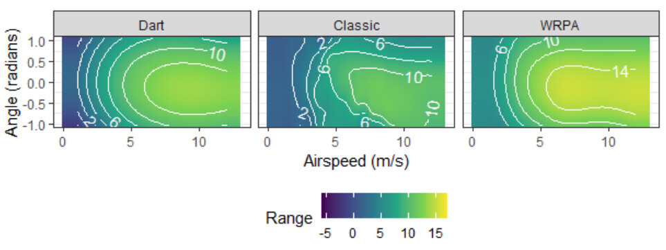
Figure 4-1: GP interpolation of terminal range of three paper airplane models, as predicted by an ordinary differential equation solver.
The GP was the right tool for the deterministic simulation, but when they fit a GAM to the outputs of the stochastic version of the paper airplane simulation,6 the GAM isolated factor effects and generated visualizations that analysts could more easily understand, compared to the full interaction surface generated by the GP. We show the decomposition of the effects into additive parts in Figure 4-2, and the response surface (the sum of the functions and the effects for the model) in Figure 4-3. This would matter for analysts looking to judge whether outputs generated by an M&S tool are reasonable at face value.
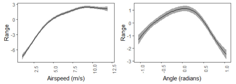
Figure 4-2: GAM component functions of a fit to (random) terminal range outputs from a paper airplane simulation. For a given combination of initial (mean) airspeed and angle, one adds the value of the function with the average for an airplane model (9.3m for Dart, 7.4m for Classic, 11.3m for WRPA) to generate a predicted terminal range. Error regions are displayed in grey.
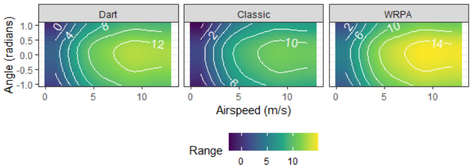
Figure 4-3: The GAM-estimated response surface for mean terminal range of three different paper airplane models given initial (mean) angle and airspeed. The plots shown here are the sum of the functions and airplane model averages in Figure 4-2
Statistical procedures determine whether a metamodel describes outputs well
After estimating the metamodel, analysts must evaluate metamodel performance using outputs other than those used to estimate the metamodel. We recommend characterizing final metamodel predictive ability with its performance in an evaluation output set. Splitting methods, such as using a screening output set and applying cross-validation, help analysts decide which statistical modeling strategy to apply (Hastie, Tibshirani and Friedman 2009). Statistical model performance metrics, such as mean-square error, accuracy, and many others described by Haman and Miller (2023), help quantify metamodel predictive performance. Visualizations comparing predicted values to observed outcomes also help analysts understand how well a metamodel makes predictions; we show such a plot for the aforementioned paper airplane terminal range metamodel in Figure 5-1. In this example, the metamodel’s predictions in the evaluation set are about as accurate as they were in the training data, implying the metamodel generalizes to unseen outputs well. A statistical test, checking if a one-to-one relationship between observed and predicted output describes the outputs on average, agrees with this visual assessment.
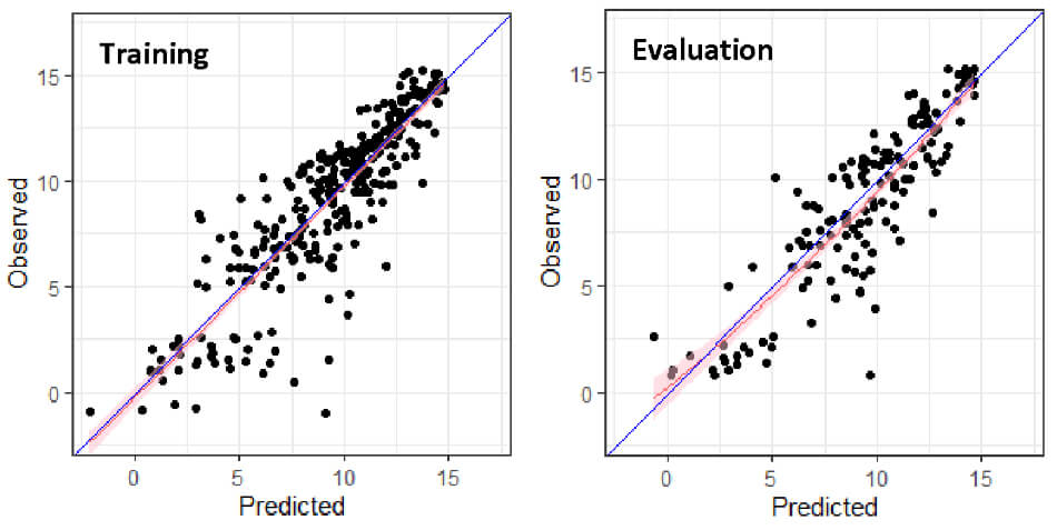
Figure 5-1: Plots comparing the predictions of the metamodel visualized in Figure 4-2 and Figure 4-3 to corresponding observed outputs; the blue line represents the ideal one-to-one relationship between predicted and observed response, and the red line with shaded region estimates the true relationship between observed and predicted response. Dots are observations. The plot on the left visualizes outputs used for training the metamodel; this plot should always look good. The plot on the right is for outputs in the evaluation set, unseen in metamodel training and thus indicative of the metamodel’s ability to generalize beyond its training set. The plots look almost equally good, suggesting the metamodel generalizes to unseen outputs well.
The authors used the design shown in Figure 3-4 to fit a statistical metamodel. Not shown are the two designs used for studying a metamodel’s performance when it is fed out-of-sample observations. One of the two designs, called the screening design, provides intermediate evaluations of a metamodel’s out-of-sample performance and can help pick a model based on that performance. They used the other design, called the evaluation design, for a final estimate and to characterize out-of-sample performance; by the time that design is used, the statistical model has been estimated and will not be revisited. This splitting strategy, incorporated into the overall DOE, ensures good estimates of out-of-sample performance, which helps ensure that the resulting metamodel’s predictions generalize beyond the outputs used for estimation. In other words, the strategy reduces the risk of overfitting, or estimating a statistical metamodel that predicts the observed outputs well but generalizes poorly beyond the sample used for estimation.
After estimating a metamodel and gaining confidence that it describes M&S outputs well, we can use it for our intended purpose. In the OT and V&V context, that includes
- predicting system performance;
- quantifying the variability and uncertainty in M&S outputs (via statistical testing and confidence intervals);
- face-value M&S quality judgements (do M&S outputs make sense?);
- comparison to live test data; and
- finding regions of interest for live testing and recommending statistical models for test planning
Conclusion
The push by operational testers to use M&S creates a corresponding need for statistical methods equipped to characterize M&S predictions well and compare those predictions to live test data. The standards set out in DOT&E’s 2016 and 2017 memos are good criteria for quality M&S analysis. The goal of this paper is to provide information to help testers implement the DOT&E guidance. We hope that, as a result, M&S outputs will lead to easier and better OT assessments of systems and equipment.
Acknowledgements
We thank Dr. John Haman, an IDA research staff member and leader of the project that generated this paper. Dr. Rebecca Medlin, another IDA research staff member, made significant contributions as well. Dr. Jeremy Werner, science advisor at DOT&E, sponsored the effort leading to this paper and offered valuable input. A number of IDA internal technical reviewers also provided valuable feedback. We also thank the referees for this paper for their input which improved this paper’s quality.
References
Ba, Shan, William R. Myers, and William A. Brenneman. 2015. “Optimal sliced Latin hypercube designs.” Technometrics 57 (4): 479-487.
Damblin, Guillaume, Mathieu Couplet, and Bertrand Iooss. 2013. “Numerical studies of space-filling designs: optimization of Latin Hypercube Samples and subprojection properties.” Journal of Simulation 7 (4): 276–289.
Director, Operational Test and Evaluation. 2017. “Clarifications on Guidance on the Validation of Models and Simulation used in Operational Test and Live Fire Assessments.” Washington, District of Columbia, January 17. https://www.dote.osd.mil/Portals/97/pub/policies/2017/20170117_Clarification_on_Guidance_on_the_Validation_of_ModSim_used_in_OT_and_LF_Assess(15520).pdf?ver=2019-08-19-144121-123.
- “Guidance on the Validation of Models and Simulation used in Operational Test and Live Fire Assessments.” Memorandum. Washington, District of Columbia, March 14. https://www.dote.osd.mil/Portals/97/pub/policies/2016/20140314_Guidance_on_Valid_of_Mod_Sim_used_in_OT_and_LF_Assess_(10601).pdf?ver=2019-08-19-144201-107.
Gramacy, Robert B. 2020. Surrogates: Gaussian Process Modeling, Design, and Optimization for the Applied Sciences. Boca Raton, Florida: CRC Press.
Haman, John T., and Curtis G. Miller. 2023. Metamodeling Techniques for Verification and Validation of Modeling and Simulation Data. Paper, Alexandria, Virginia: Institute for Defense Analyses.
Hastie, Trevor, Robert Tibshirani, and Jerome Friedman. 2009. The Elements of Statistical Learning: Data Mining, Inference, and Prediction. 2. New York, New York: Springer.
Lekivetz, Ryan, and Bradley Jones. 2019. “Fast Flexible Space-Filling Designs with Nominal Factors for Nonrectangular Regions.” Quality and Reliability Engineering International 35 (2): 677-684.
Roshan, Joseph V., Evren Gul, and Shan Ba. 2015. “Maximum Projection Designs for Computer Experiments.” Biometrika 102 (2): 317-380.
Wojton, Heather M., Kelly M. Avery, Han G. Yi, and Curtis G. Miller. 2021. Space filling designs for modeling & simulation validation. Paper, Alexandria, Virginia: Institute for Defense Analyses.
Wood, Simon N. 2017. Generalized Additive Models: An Introduction with R. 2. Boca Raton, Florida: CRC Press.
Acronyms
DoD Department of Defense
DOE Design of Experiments
DOT&E Director, Operational Test and Evaluation
FFF Fast Flexible Filling
GAM Generalized Additive Model
GP Gaussian Process
IDA Institute for Defense Analyses
LHS Latin Hypercube Sampling
M&S Modeling and Simulation
OT Operational Test
SFD Space Filling Design
SLHS Sliced LHS
T&E Test and Evaluation
V&V Verification and Validation
WRPA World Record Paper Airplane
Endnotes
1 In the statistics community, metamodels are known as statistical emulators.
2 Replication is not a strict requirement of statistical modeling when continuous factors are present. For linear statistical models, all that is required is that the design matrix be full rank, a requirement not dependent on replication. Most optimal designs involve replicates when they have continuous factors because doing so is easier to execute and minimizes the standard errors of model parameter estimates.
3 The paper airplane flight simulation consists of a numerical ordinary differential equation solver written using the R scripting language. Stengel (2004) presents the formulas describing the flight dynamics of a paper airplane.
4 Statistical methods can incorporate physics models, known up to missing parameters, in estimation. Nonlinear statistical regression techniques do so, for instance.
5 For statistical purposes, an M&S tool that uses a seed for pseudorandom number generation is considered stochastic, despite the fact that the M&S will produce identical results given identical seeds and only emulates randomness.
6 The stochastic version of the simulation randomized initial angle and airspeed so that the specified initial angles and airspeeds were averages rather than the values fed in, simulating the possibility of error in the toss of the plane.
Author Biographies
Dr. Curtis Miller is a research staff member of the Operational Evaluation Division at the Institute for Defense Analyses. In that role, he advises analysts on effective use of statistical techniques, especially pertaining to modeling and simulation activities and U.S. Navy operational test and evaluation efforts, for the division’s primary sponsor, the Director of Operational Test and Evaluation. He obtained a PhD in mathematics from the University of Utah.